单变量线性回归
- 单变量指的是输入特征只有一个的时候,单变量线性回归数学公式及讲解文档在这里,可点击访问。
- 根据吴恩达老师的机器学习课程推荐,机器学习研究最好使用
octave/matlab作为工具,后续转成其他语言也方便,最重要的是学习其本质。
绘图
首先学会简单的绘图,基本的octave/matlab知识我是根据易百教程,这个网站了解并入门的。
plotData.m 这个文件可以实现简单的绘图功能,写成函数,方便后面直接调用。
function plotData (x, y)

figure; %open a new figure window

plot(x, y, 'rx', 'MarkerSize', 10);
ylabel('Profit in $10.000s');
xlabel('Population of city in 10,000');

endfunction
代价函数及梯度下降
computeCost.m 用来计算代价函数
也可参考上面文档中的公式:
function J = computeCost (X, y, theta)

m = length(y);
J = 0;
J = sum((X * theta - y).^2) / (2*m);

endfunction
gradientDescent.m 梯度下降函数:
做梯度下降的同时用J_history记录了每次代价函数的值:
function [theta, J_history] = gradientDescent (X, y, theta, alpha, num_iters)

m = length(y);
J_history = zeros(num_iters, 1);
thetas = theta;
for iter = 1 : num_iters
    theta(1) = theta(1) - alpha / m * sum(X * thetas - y);
    theta(2) = theta(2) - alpha / m * sum((X * thetas - y) .* X(:,2));
    thetas = theta;
    J_history(iter) = computeCost(X, y, theta);
end

endfunction
可视化
现在综合上述函数进行可视化,直观的观察数据,数据ex1data1.txt点击可下载 进行测试,使用octave/matlab执行以下命令:
%% Exercise 1: Linear Regression

%% ========== 1.Plotting ==========
data = load('ex1data1.txt');
X = data(:, 1);
y = data(:, 2);
m = length(y);
plotData(X, y);
fprintf('Program paused, Press enter to continue.\n');
pause;
原始训练数据用展示如下

image.png
%% ========== 2.Cost and Gradient descent ==========
X = [ones(m, 1), data(:, 1)];
theta = zeros(2, 1);
iterations = 2000;
alpha = 0.01;
J = computeCost(X, y, theta);
fprintf('size of X = %f\n', size(X));
fprintf('size of theta = %f\n', size(theta));
fprintf('With theta = [0; 0]\nCost computed = %f\n', J);
fprintf('Expected cost value (approx) 32.07\n');

J = computeCost(X, y, [-1; 2]);
fprintf('With theta = [-1; 2]\nCost computed = %f\n', J);
fprintf('Expected cost value (approx) 54.24\n');
fprintf('Program paused, Press enter to continue.\n');
pause

[theta, J_history] = gradientDescent(X, y, theta, alpha, iterations);
fprintf('Theta found by gradient descent:\n');
fprintf('%f\n', theta);
fprintf('Expected theta values (approx)\n');
fprintf(' -3.6303\n  1.1664\n\n');

hold on; % keep previous plot visible
plot(X(:,2), X * theta, '-');
legend('Training data', 'Linear regression');
hold off;

image.png
以下是随着迭代次数的增加代价函数减少
fprintf('%f\n', size(J_history));
figure; %open a new figure window
plot([1:size(J_history)], J_history);
pause;

predict1 = [1, 3.5] * theta;
predict2 = [1, 7] * theta;
fprintf('predict1:%f \n', predict1);
fprintf('predict2:%f \n', predict2);
fprintf('Program paused. Press enter to continue.\n');
pause;
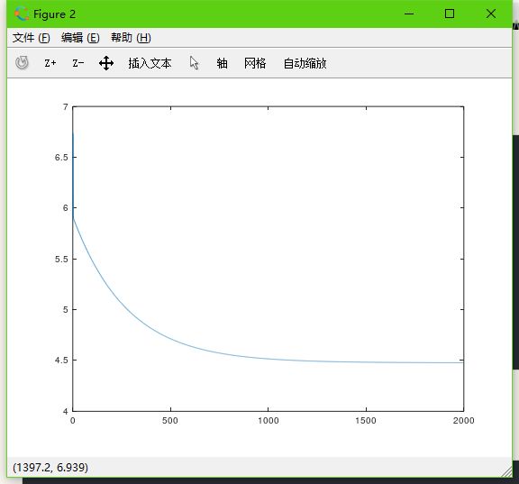
image.png
%% ========= 3.Visualizing J(theta_0, theta_1) ==========
theta0_vals = linspace(-10, 10, 100);
theta1_vals = linspace(-1, 4, 100);
J_vals = zeros(length(theta0_vals), length(theta1_vals));
for i = 1:length(theta0_vals)
    for j = 1:length(theta1_vals)
        t = [theta0_vals(i); theta1_vals(j)];
        J_vals(i,j) = computeCost(X, y, t);
    end
end

J_vals = J_vals'; %由于meshgrids在surf命令中的工作方式,我们需要在调用surf之前调换J_vals,否则轴会被翻转
% Surface plot
figure;
surf(theta0_vals, theta1_vals, J_vals); % surf命令绘制得到的是着色的三维曲面。
xlabel('\theta_0');ylabel('\theta_1');
% Contour plot
figure;
contour(theta0_vals, theta1_vals, J_vals, logspace(-2, 3, 20)); % contour用来绘制矩阵数据的等高线
xlabel('\theta_0');ylabel('\theta_1');
hold on;
plot(theta(1), theta(2), 'rx', 'MarkerSize', 10, 'LineWidth', 2);

image.png
等高线:

image.png