一、背景
1.公司大量优秀且有经验的员工过早的离开
2.数据来源:kaggle
3.变量
satisfaction: Employee satisfaction level
evaluation: Last evaluation
project: Number of projects
hours: Average monthly hours
years: Time spent at the company
accident: Whether they have had a work accident
promotion: Whether they have had a promotion in the last 5 years
sales: Department
salary: Salary
left: Whether the employee has left
4.分析目的与衡量标准:
(1)分析并得出优秀员工离职的主要可能的原因
(2)构建预测模型,预测下一位将会离开的优秀员工是谁
二、数据分析
所需包导入
library(readr)
library(dplyr)
library(ggplot2)
library(gmodels)
(一)导入数据并查看
## 1.1 数据导入
library(readr)
hr <- read_csv("HR_comma_sep.csv")
hr <- tbl_df(hr)
View(hr)
str(hr)
Classes ‘tbl_df’, ‘tbl’ and 'data.frame': 14999 obs. of 10 variables:
$ satisfaction_level : num 0.38 0.8 0.11 0.72 0.37 0.41 0.1 0.92 0.89 0.42 ...
$ last_evaluation : num 0.53 0.86 0.88 0.87 0.52 0.5 0.77 0.85 1 0.53 ...
$ number_project : int 2 5 7 5 2 2 6 5 5 2 ...
$ average_montly_hours : int 157 262 272 223 159 153 247 259 224 142 ...
$ time_spend_company : int 3 6 4 5 3 3 4 5 5 3 ...
$ Work_accident : int 0 0 0 0 0 0 0 0 0 0 ...
$ left : int 1 1 1 1 1 1 1 1 1 1 ...
$ promotion_last_5years: int 0 0 0 0 0 0 0 0 0 0 ...
$ sales : chr "sales" "sales" "sales" "sales" ...
$ salary : chr "low" "medium" "medium" "low" ...
## 1.2 变量重命名
hr_good <- filter(hr, evaluation>=0.75 & year>=4 & project>= 4)
colnames(hr) <- c("satisfaction","evaluation","project","hours","years","accident","left","promotion","sales","salary")
## 1.3 因子化
hr$sales <- factor(hr$sales)
hr$salary <- factor(hr$salary, levels=c("low","medium","high"))
## 1.4 查看数据
sum(is.na(hr))
# [1] 0
summary(hr)
satisfaction_level last_evaluation number_project average_montly_hours
Min. :0.0900 Min. :0.3600 Min. :2.000 Min. : 96.0
1st Qu.:0.4400 1st Qu.:0.5600 1st Qu.:3.000 1st Qu.:156.0
Median :0.6400 Median :0.7200 Median :4.000 Median :200.0
Mean :0.6128 Mean :0.7161 Mean :3.803 Mean :201.1
3rd Qu.:0.8200 3rd Qu.:0.8700 3rd Qu.:5.000 3rd Qu.:245.0
Max. :1.0000 Max. :1.0000 Max. :7.000 Max. :310.0
time_spend_company Work_accident left promotion_last_5years
Min. : 2.000 Min. :0.0000 Min. :0.0000 Min. :0.00000
1st Qu.: 3.000 1st Qu.:0.0000 1st Qu.:0.0000 1st Qu.:0.00000
Median : 3.000 Median :0.0000 Median :0.0000 Median :0.00000
Mean : 3.498 Mean :0.1446 Mean :0.2381 Mean :0.02127
3rd Qu.: 4.000 3rd Qu.:0.0000 3rd Qu.:0.0000 3rd Qu.:0.00000
ax. :10.000 Max. :1.0000 Max. :1.0000 Max. :1.00000
sales salary
sales :4140 low :7316
technical :2720 medium:6446
support :2229 high :1237
IT :1227
product_mng: 902
marketing : 858
(Other) :2923
(二)根据定义选取优秀员工的子集,并做初步分析
优秀员工的定义:
(1)评价(evaluation)>=0.75
(2)项目数量(project)>=4
(3)有经验的(year)>=4
## 2.1 根据定义选取子集
hr_good <- filter(hr, evaluation>=0.75 & years>=4 & project>= 4)
## 2.2 对比总体与选取子集中离职员工的占比情况
【结论】:优秀员工离职情况非常严重
1.在总离职员工中,优秀员工的数量占了(1778/3571=) 50%;
2.在优秀员工子集中,离职的数量高达(1778/2753=) 64%;
CrossTable(hr$left)
Total Observations in Table: 14999
| stay | left |
|-----------|-----------|
| 11428 | 3571 |
| 0.762 | 0.238 |
|-----------|-----------|
CrossTable(hr_good$left)
Total Observations in Table: 2763
| stay | left |
|-----------|-----------|
| 985 | 1778 |
| 0.356 | 0.644 |
|-----------|-----------|
## 2.3 了解优秀员工子集的统计量
summary(hr_good)
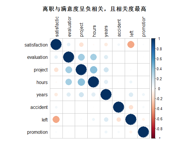
## 2.4 了解优秀员工子集中各变量之间的相关性
【结论】:离职与满意度呈负相关,且相关度最高
hr_good_corr <- select(hr, -sales,-salary) %>% cor()
corrplot(hr_good_corr, method="circle", tl.col="black",title="离职与满意度呈负相关,且相关度最高",mar=c(1,1,3,1))
(三)逐个变量分析员工离职、满意度与其他变量之间的关系
## 3.1 查看满意度的分布图
hr_good$left <- factor(hr_good$left, levels=c(0,1), labels=c("stay", "left"))
ggplot(hr_good, aes(satisfaction, fill=left)) + geom_histogram(position="dodge") + scale_x_continuous(breaks=c(0.1,0.13,0.25,0.50,0.73,0.75,0.92,1.00)) + theme3 + theme(axis.text.x=element_text(angle=90)) + labs(title="满意度在[0.1,0.13]与[0.73,0.92]两个区间离职人数非常多")

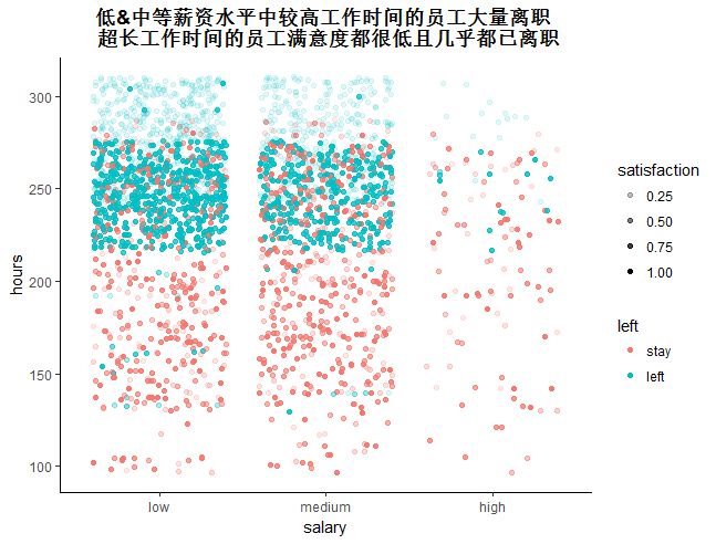
## 3.2 收入、工作时间、满意度之间的关系
【结论】:工作超长时间的员工满意度低,且离职率高
1.低&中等薪资水平中较高工作时间的员工大量离职
2.超长工作时间的员工满意度都很低且几乎都已离职
ggplot(hr_good, aes(salary, hours, alpha=satisfaction, color=left)) + geom_jitter() + theme3 + labs(title=paste("低&中等薪资水平中较高工作时间的员工大量离职","\n","超长工作时间的员工满意度都很低且几乎都已离职"))
## 3.3 晋升、满意度与离职的关系
【结论】:高评价的员工几乎没有人晋升,离职人员也主要集中在未晋升中
ggplot(hr_good, aes(promotion, evaluation, color=left)) + geom_jitter() + theme3 + scale_x_discrete(limits=c(0,1)) + labs(title=paste("高评价的员工几乎没有人晋升","\n","离职人员也主要集中在未晋升中"))

## 3.4 工作年限、满意度与离职的关系
【结论】:
1.低满意度(0.1)水平下,4年司龄的员工大量离职
2.大量高满意度员工在第5年与第6年离职
3.7年以上的员工没有人离职
ggplot(hr_good, aes(years,satisfaction, color=left)) + geom_jitter() + scale_x_discrete(limits=c(4,5,6,7,8,9,10)) + theme3 + labs(title=paste("低满意度(","0.1)","水平下,4年司龄的员工大量离职","\n","大量高满意度员工在第5年与第6年离职"))

## 3.5 部门、项目数与离职的关系
【结论】:对于6个以上的项目无论在哪个部门离职率都非常高
ggplot(hr_good, aes(sales,fill=left)) + geom_bar(position="fill") + facet_wrap(~factor(project),ncol=1) + theme3 + theme(axis.text.x=element_text(angle=270)) + labs(y="number projcet",title="对于6个以上的项目无论在哪个部门离职率都非常高")

## 3.6 部门与离职的关系
【结论】:各部门离职人员均高于在职人员,管理部门除外
ggplot(hr_good, aes(sales, fill=left)) + geom_bar(position="dodge") + coord_flip() + scale_x_discrete(limits=c("management","RandD","hr","accounting","marketing","product_mng","IT","support","technical","sales")) + labs(title="各部门离职人员均高于在职人员,管理部门除外") + theme3

三、构建预测模型1:分类
## 数据分割
library(caret)
set.seed(0001)
train <- createDataPartition(hr_good$left, p=0.75, list=FALSE)
hr_good_train <- hr_good[train, ]
hr_good_test <- hr_good[-train, ]
(一)Logistic回归
## 1. 构建逻辑回归并验证
ctrl <- trainControl(method="cv",number=5)
logit <- train(left~., hr_good_train, method="LogitBoost", trControl=ctrl)
logit.pred <- predict(logit, hr_good_test, tyep="response")
confusionMatrix( hr_good_test$left, logit.pred)
Confusion Matrix and Statistics
Reference
Prediction stay left
stay 213 33
left 8 436
Accuracy : 0.9406
95% CI : (0.9203, 0.957)
No Information Rate : 0.6797
P-Value [Acc > NIR] : < 2.2e-16
Kappa : 0.8675
Mcnemar's Test P-Value : 0.0001781
Sensitivity : 0.9638
Specificity : 0.9296
Pos Pred Value : 0.8659
Neg Pred Value : 0.9820
Prevalence : 0.3203
Detection Rate : 0.3087
Detection Prevalence : 0.3565
Balanced Accuracy : 0.9467
'Positive' Class : stay
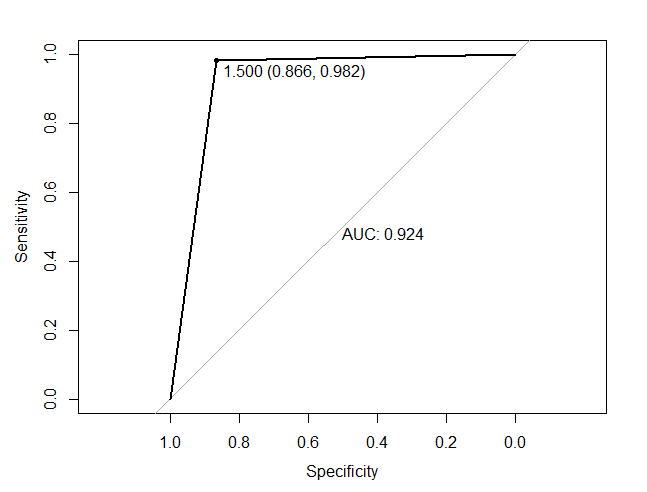
## 2. 评价模型,绘制ROC/AUC曲线
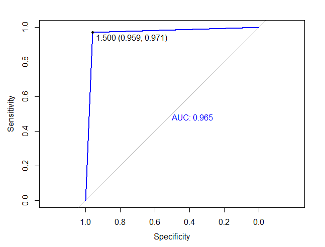
library(pROC)
roc(as.numeric(hr_good_test$left), as.numeric(logit.pred), plot=TRUE, print.thres=TRUE, print.auc=TRUE, col="black")
(二)决策树
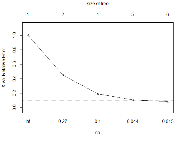
## 1. 构建决策树
library(rpart)
dtree <- rpart(left~., hr_good_train, method="class",parms=list(split="information"))
dtree$cptable
CP nsplit rel error xerror xstd
1 0.55209743 0 1.00000000 1.00000000 0.02950911
2 0.12855210 1 0.44790257 0.44790257 0.02256805
3 0.08254398 3 0.19079838 0.19079838 0.01551204
4 0.02300406 4 0.10825440 0.10825440 0.01186737
5 0.01000000 5 0.08525034 0.08525034 0.01057607
plotcp(dtree)
dtree.pruned <- prune(dtree, cp=0.01)
library(partykit)
library(grid)
plot(as.party(dtree.pruned),main="Decision Tree")

dtree.pruned.pred <- predict(dtree.pruned, hr_good_test, type="class")
confusionMatrix(hr_good_test$left, dtree.pruned.pred)
Confusion Matrix and Statistics
Reference
Prediction stay left
stay 236 10
left 13 431
Accuracy : 0.9667
95% CI : (0.9504, 0.9788)
No Information Rate : 0.6391
P-Value [Acc > NIR] : <2e-16
Kappa : 0.9275
Mcnemar's Test P-Value : 0.6767
Sensitivity : 0.9478
Specificity : 0.9773
Pos Pred Value : 0.9593
Neg Pred Value : 0.9707
Prevalence : 0.3609
Detection Rate : 0.3420
Detection Prevalence : 0.3565
Balanced Accuracy : 0.9626
'Positive' Class : stay
## 2. 评价模型,绘制ROC/AUC曲线
roc(as.numeric(hr_good_test$left),as.numeric(dtree.pruned.pred), plot=TRUE, print.thres=TRUE, print.auc=TRUE,col="blue")
(三)随机森林
## 1. 构建随机森林
library(randomForest)
set.seed(0002)
forest <- randomForest(left~., hr_good_train, importance=TRUE, na.action=na.roughfix)
forest
Call:
randomForest(formula = left ~ ., data = hr_good_train, importance = TRUE, na.action = na.roughfix)
Type of random forest: classification
Number of trees: 500
No. of variables tried at each split: 3
OOB estimate of error rate: 1.35%
Confusion matrix:
stay left class.error
stay 731 8 0.01082544
left 20 1314 0.01499250
importance(forest, type=2)
MeanDecreaseGini
satisfaction 315.455428
evaluation 63.101527
project 51.659717
hours 307.201129
years 168.530576
accident 6.232136
promotion 1.897123
sales 20.666829
salary 12.338717
forest.pred <- predict(forest, hr_good_test)
confusionMatrix(hr_good_test$left, forest.pred)
Confusion Matrix and Statistics
Reference
Prediction stay left
stay 241 5
left 4 440
Accuracy : 0.987
95% CI : (0.9754, 0.994)
No Information Rate : 0.6449
P-Value [Acc > NIR] : <2e-16
Kappa : 0.9715
Mcnemar's Test P-Value : 1
Sensitivity : 0.9837
Specificity : 0.9888
Pos Pred Value : 0.9797
Neg Pred Value : 0.9910
Prevalence : 0.3551
Detection Rate : 0.3493
Detection Prevalence : 0.3565
Balanced Accuracy : 0.9862
'Positive' Class : stay
## 2. 评价模型,绘制ROC/AUC曲线
roc(as.numeric(hr_good_test$left), as.numeric(forest.pred), plot=TRUE, print.thres=TRUE, print.auc=T, col="green")

(四)支持向量机SVM
## 1. 构建SVM
library(e1071)
set.seed(0003)
svm <- svm(left~., hr_good_train)
svm.pred <- predict(svm, na.omit(hr_good_test))
confusionMatrix(na.omit(hr_good_test)$left, svm.pred)
Confusion Matrix and Statistics
Reference
Prediction stay left
stay 211 35
left 11 433
Accuracy : 0.9333
95% CI : (0.9121, 0.9508)
No Information Rate : 0.6783
P-Value [Acc > NIR] : < 2.2e-16
Kappa : 0.8515
Mcnemar's Test P-Value : 0.000696
Sensitivity : 0.9505
Specificity : 0.9252
Pos Pred Value : 0.8577
Neg Pred Value : 0.9752
Prevalence : 0.3217
Detection Rate : 0.3058
Detection Prevalence : 0.3565
Balanced Accuracy : 0.9378
'Positive' Class : stay
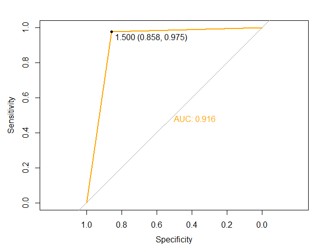
## 2. 评价模型,绘制ROC/AUC曲线
roc(as.numeric(na.omit(hr_good_test)$left), as.numeric(svm.pred), plot=T, print.thres=T, print.auc=T, col="orange")
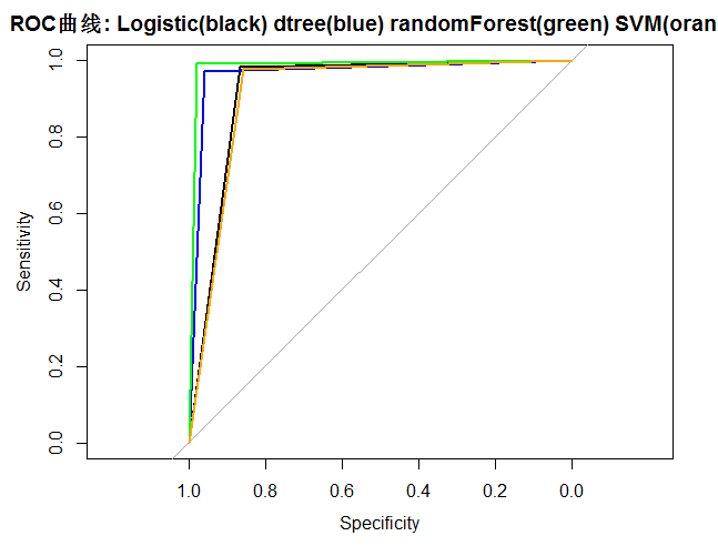
(五)对比模型,选择准确性最高的模型
【结论】:随机森林的拟合度最高,选择该模型为预测模型
roc(as.numeric(hr_good_test$left), as.numeric(logit.pred), plot=TRUE,col="black",main=paste("ROC曲线:","Logitis(black)","dtree(blue)","randomForest(green)","SVM(orange)",sep=" "))
roc(as.numeric(hr_good_test$left),as.numeric(dtree.pruned.pred), plot=TRUE, col="blue", add=T)
roc(as.numeric(hr_good_test$left), as.numeric(forest.pred), plot=TRUE, col="green", add=T)
roc(as.numeric(na.omit(hr_good_test)$left), as.numeric(svm.pred), plot=T, col="orange", add=T)
(六)模型应用
importance(forest,type=2)
MeanDecreaseGini
satisfaction 315.455428
evaluation 63.101527
project 51.659717
hours 307.201129
years 168.530576
accident 6.232136
promotion 1.897123
sales 20.666829
salary 12.338717
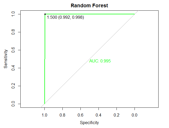
## 1. 剔除明显不重要的因子,重新构建模型
forest2 <- randomForest(left~.-promotion-accident-salary-sales, hr_good, na.action=na.roughfix, importance=TRUE)
importance(forest2, type=2)
MeanDecreaseGini
satisfaction 462.97925
evaluation 72.49430
project 71.09463
hours 417.63782
years 231.64080
forest2.pred <- predict(forest2, hr_good_test)
confusionMatrix(hr_good_test$left, forest2.pred, positive="left")
Confusion Matrix and Statistics
Reference
Prediction stay left
stay 244 2
left 1 443
Accuracy : 0.9957
95% CI : (0.9873, 0.9991)
No Information Rate : 0.6449
P-Value [Acc > NIR] : <2e-16
Kappa : 0.9905
Mcnemar's Test P-Value : 1
Sensitivity : 0.9959
Specificity : 0.9955
Pos Pred Value : 0.9919
Neg Pred Value : 0.9977
Prevalence : 0.3551
Detection Rate : 0.3536
Detection Prevalence : 0.3565
Balanced Accuracy : 0.9957
'Positive' Class : stay
## 2. 评价模型,绘制ROC/AUC曲线
roc(as.numeric(hr_good_test$left), as.numeric(forest2.pred), plot=TRUE, print.thres=T, print.auc=T, main="Random Forest", col="green")
(七)结论
1.调整后的随机森林预测模型员工离职的准确性达99.5%;其中离职的员工被正确预测的概率为99.5%,被预测离职的员工中,实际离职的概率为99.8%;
2.剔除不重要的变量(promotion,accident,sales,salary)并不会对模型造成影响;
3.满意度(satisfaction)、月平均工作时间(hours)、工作年限(years)是影响优秀员工离职的主要三个变量