情感分析之电影评论分析-基于Tensorflow的LSTM
1. 深度学习在自然语言处理中的应用
自然语言处理是教会机器如何去处理或者读懂人类语言的系统,目前比较热门的方向,包括如下几类:
对话系统 - 比较著名的案例有:Siri,Alexa 和 Cortana。
情感分析 - 对一段文本进行情感识别。
图文映射 - 用一句话来描述一张图片。
机器翻译 - 将一种语言翻译成另一种语言。
语音识别 - 让电脑识别口语。
2. 情感分析基本方法
目前对情感分析的研究主要集中在两个方面:识别给定的文本实体是主观的还是客观的,以及识别主观的文本的极性。大多数情感分析研究都使用机器学习方法。
分析方法主要有以下三种:
- 词法分(基于词典的打分机制)
- 基于机器学习的分析
- 混合分析
下面简单介绍下这三种方法:
- 词法分析
词法分析运用了由预标记词汇组成的字典,使用词法分析将器将输入文本转化为单词序列。将新的单词与词典中的词汇进行匹配。如果有一个积极的匹配,正分数就加到分数总池中。如果有一个消极的匹配,输入文本的总分数就会减少。最后文本的分类就取决于文本的总得分。目前有大量的工作致力于度量词法信息的有效性。 - 机器学习方法
机器学习具有高的适应性和准确性,也因此受到了越来越多的关注。在情感分析中主要使用的是监督学习方法。可以分为三个阶段:数据收集、预处理、训练分类。并且在训练过程中,需要提供一个标记语料库作为训练数据。分类器使用一系列特征向量对目标数据进行分类。 - 混合分析
目前情感分析研究将两种方法进行组合,这样既可以利用机器学习方法的高准确性,又可以利用词法分析的快速的特性。有研究者利用由两个词组成的词汇和一个未标记的数据作为训练集。思想是:首先将这些由两个词组成的词汇划分为积极的类和消极的类,然后把这些词汇集合进行向量化表示,每个类都有一个中心向量代表该类,然后计算未标记词和中心词向量之间的余弦相似度,根据相似度将该文件划分为积极和消极的类,最后把这些全部送进分类器进行分类。个人理解这里其实有点半监督学习的意思。。
3. 实战电影评论情感分析
该任务可以被认为是从一个句子,一段话,或者是从一个文档中,将作者的情感分为积极的,消极的或者中性的。这篇教程由多个主题组成,包括词向量,循环神经网络和LSTM,tensorflow框架的搭建。
3.1 关于词向量:
我们需要考虑不同形式的数据,这些数据被用来作为机器学习或者深度学习模型的输入数据。卷积神经网络使用像素值作为输入,logistic回归使用一些可以量化的特征值作为输入,强化学习模型使用奖励信号来进行更新。通常的输入数据是需要被标记的标量值。
词向量模型:
我们可以将一句话中的每一个词都转换成一个向量:输入数据可以看成是一个 16*D 的矩阵

Word2Vec:
为了去得到这些词嵌入,我们使用模型 “Word2Vec”。简单的说,这个模型根据上下文的语境来推断出每个词的词向量。如果两个个词在上下文的语境中,可以被互相替换,那么这两个词的距离就非常近。在自然语言中,上下文的语境对分析词语的意义是非常重要的。这个模型的作用就是从一大堆句子(以 Wikipedia 为例)中为每个独一无二的单词进行建模,并且输出一个唯一的向量。Word2Vec 模型的输出被称为一个嵌入矩阵。

这个嵌入矩阵包含训练集中每个词的一个向量。传统来讲,这个嵌入矩阵中的词向量数据会很大。
Word2Vec 模型根据数据集中的每个句子进行训练,并且以一个固定窗口在句子上进行滑动,根据句子的上下文来预测固定窗口中间那个词的向量。然后根据一个损失函数和优化方法,来对这个模型进行训练。
具体的可以参考:
https://blog.csdn.net/lilong117194/article/details/82182869
https://blog.csdn.net/lilong117194/article/details/81979522
3.2 循环神经网络和LSTM
这方面的资料很多,这里不再重复讲lstm相关的知识。
3.3 代码实现
有了上面的基础,下面就进行贴出代码,整体流程如下:
1) 制作词向量,可以使用gensim这个库,也可以直接用现成的训练好的
2) 词和ID的映射
3) 构建RNN网络架构
4) 训练模型
5) 测试模型效果
整体的代码为:
#!/usr/bin/env python3
# -*- coding: utf-8 -*-
"""
Created on Wed Aug  8 14:13:14 2018
@author: lilong
"""

import numpy as np
import time
import datetime
import os
import re
from random import randint
from os.path import isfile, join
import tensorflow as tf


"""
使用训练好的词向量模型,该矩阵包含400000x50的数据;还有一个是400000的词典
"""

wordsList = np.load('wordsList.npy')
print('载入word列表:',np.shape(wordsList),type(wordsList))
# 这里转化为列表,但是是[b'and', b'in', b'a', b'"', b"'s", b'for']的形式,即是二进制编码。
wordsList = wordsList.tolist()
# 转化为utf-8编码的形式,['of', 'to', 'and', 'in', 'a', '"', "'s", 'for', '-',]
wordsList = [word.decode('UTF-8')  for word in wordsList]
# 400000x50的嵌入矩阵,这个是训练好的词典向量模型
wordVectors = np.load('wordVectors.npy')
print('载入文本向量:',wordVectors.shape)
#print(wordVectors[home_ndex]) # 得到对应词典中词的50维向量


"""
解析文件,数据预处理,得到正负评价下的文件
"""

# 这里得到了所有的正面评价文件夹pos下的文件路径
pos_files = ['pos/' + f
             for f in os.listdir('pos/')
                 if isfile(join('pos/', f))]
# 这里得到了所有的neg文件夹下的文件路径
neg_files = ['neg/' + f
             for f in os.listdir('neg/')
                 if isfile(join('neg/', f))]
num_words = []
# 这里的每个txt文件都是一行文本,12500都是正面评价
for pf in pos_files:
    with open(pf, "r", encoding='utf-8') as f:
        line = f.readline()
        counter = len(line.split())
        num_words.append(counter)
print('正面评价完结。。。')
# 这里是12500负面评价
for nf in neg_files:
    with open(nf, "r", encoding='utf-8') as f:
        line = f.readline()
        counter = len(line.split())
        num_words.append(counter)
print('负面评价完结。。。')
num_files = len(num_words)
print('文件总数:', num_files)
print('所有的词的数量:', sum(num_words))
print('平均文件的词的长度:', sum(num_words) / len(num_words))


"""
辅助函数:返回一个数据集的迭代器,用于返回一批训练集合

"""
max_seq_num = 250
num_dimensions = 50  # 每个单词向量的维度,这里和嵌入矩阵的每个词的维度相同

# arr:24 x 250的矩阵
def get_train_batch():
    labels = []
    arr = np.zeros([batch_size, max_seq_num])
    for i in range(batch_size):
        if (i % 2 == 0):
            num = randint(1, 11499)
            labels.append([1, 0])
        else:
            num = randint(13499, 24999)
            labels.append([0, 1])
        arr[i] = ids[num - 1:num]
    return arr, labels

# 同上
def get_test_batch():
    labels = []
    arr = np.zeros([batch_size, max_seq_num])
    for i in range(batch_size):
        num = randint(11499, 13499)
        if (num <= 12499):
            labels.append([1, 0])
        else:
            labels.append([0, 1])
        arr[i] = ids[num - 1:num]
    return arr, labels


"""
构建tensorflow图

"""

batch_size = 24 # batch的尺寸
lstm_units = 64 # lstm的单元数量
num_labels = 2  # 输出的类别数
iterations = 200000 # 迭代的次数
# 载入正负样本的词典映射
ids = np.load('idsMatrix.npy')
print('载入IDS:',ids.shape)
tf.reset_default_graph()
# 确定好单元的占位符:输入是24x300,输出是24x2
labels = tf.placeholder(tf.float32, [batch_size, num_labels])
input_data = tf.placeholder(tf.int32, [batch_size, max_seq_num])

# 必须先定义该变量
data = tf.Variable(
    tf.zeros([batch_size, max_seq_num, num_dimensions]), dtype=tf.float32)
# 调用tf.nn.lookup()接口获得文本向量,该函数返回batch_size个文本的3D张量,用于后续的训练
data = tf.nn.embedding_lookup(wordVectors, input_data)

# 使用tf.contrib.rnn.BasicLSTMCell细胞单元配置lstm的数量
lstmCell = tf.contrib.rnn.BasicLSTMCell(lstm_units)
# 配置dropout参数,以此避免过拟合
lstmCell = tf.contrib.rnn.DropoutWrapper(cell=lstmCell, output_keep_prob=0.75)
# 最后将LSTM cell和数据输入到tf.nn.dynamic_rnn函数,功能是展开整个网络,并且构建一整个RNN模型
# 这里的value认为是最后的隐藏状态,该向量将重新确定维度,然后乘以一个权重加上偏置,最终获得lable
value, _ = tf.nn.dynamic_rnn(lstmCell, data, dtype=tf.float32)

weight = tf.Variable(tf.truncated_normal([lstm_units, num_labels]))
bias = tf.Variable(tf.constant(0.1, shape=[num_labels]))
value = tf.transpose(value, [1, 0, 2])
last = tf.gather(value, int(value.get_shape()[0]) - 1)
prediction = (tf.matmul(last, weight) + bias)

# 定义正确的预测函数和正确率评估参数
correctPred = tf.equal(tf.argmax(prediction, 1), tf.argmax(labels, 1))
accuracy = tf.reduce_mean(tf.cast(correctPred, tf.float32))

# 最后将标准的交叉熵损失函数定义为损失值,这里是以adam为优化函数
loss = tf.reduce_mean(tf.nn.softmax_cross_entropy_with_logits_v2(logits=prediction, labels=labels))
optimizer = tf.train.AdamOptimizer().minimize(loss)


sess = tf.InteractiveSession()
saver = tf.train.Saver()
sess.run(tf.global_variables_initializer())


tf.summary.scalar('loss',loss)
tf.summary.scalar('Accrar',accuracy)
merged=tf.summary.merge_all()
logdir='tensorboard/'+ datetime.datetime.now().strftime("%Y%m%d-%H%M%S")+"/"
writer=tf.summary.FileWriter(logdir,sess.graph)


iterations = 100000
for i in range(iterations):
    # 下个批次的数据
    next_batch, next_batch_labels = get_train_batch()
    sess.run(optimizer,{input_data: next_batch, labels: next_batch_labels})

    # 每50次写入一次leadboard
    if(i%50==0):
        summary=sess.run(merged,{input_data: next_batch, labels: next_batch_labels})
        writer.add_summary(summary,i)

    if (i%1000==0):
        loss_ = sess.run(loss, {input_data: next_batch, labels: next_batch_labels})

        accuracy_=(sess.run(accuracy, {input_data: next_batch, labels: next_batch_labels})) * 100
        print("iteration:{}/{}".format(i+1, iterations),
                  "\nloss:{}".format(loss_),
                  "\naccuracy:{}".format(accuracy_))
        print('..........')
    # 每10000次保存一下模型
    if(i%10000==0 and i!=0):
        save_path=saver.save(sess,"models/pretrained_lstm.ckpt",gloal_step=i)
        print("saved to %s"% save_path)

writer.close()
运行结果:
载入word列表: (400000,) 'numpy.ndarray'>
载入文本向量: (400000, 50)
正面评价完结。。。
负面评价完结。。。
文件总数: 25000
所有的词的数量: 5844680
平均文件的词的长度: 233.7872
载入IDS: (25000, 250)
iteration:1/100000
loss:0.7998574376106262
accuracy:58.33333134651184
..........
iteration:1001/100000
loss:0.6967594027519226
accuracy:54.16666865348816
..........
iteration:2001/100000
loss:0.6576123237609863
accuracy:62.5
..........
iteration:3001/100000
loss:0.6840474605560303
accuracy:62.5
..........
iteration:4001/100000
loss:0.6713441014289856
accuracy:58.33333134651184
..........
iteration:5001/100000
loss:0.6841540932655334
accuracy:54.16666865348816
..........
iteration:6001/100000
loss:0.7225241661071777
accuracy:66.66666865348816
..........
.
.
.
注意:这里的所有运行中用到的准备文件都是提前训练好的,下面会有介绍。
由于时间问题这里没有跑完所有的训练迭代轮数,但可以看到在每个batch下的损失率和准确率。
下面拆解整体的流程:
(1) 导入数据
首先,我们需要去创建词向量。为了简单起见,我们使用训练好的模型来创建。
作为该领域的一个最大玩家,Google 已经帮助我们在大规模数据集上训练出来了 Word2Vec 模型,包括 1000 亿个不同的词!在这个模型中,谷歌能创建 300 万个词向量,每个向量维度为 300。
在理想情况下,我们将使用这些向量来构建模型,但是因为这个单词向量矩阵相当大(3.6G),我们用另外一个现成的小一些的,该矩阵由 GloVe 进行训练得到。矩阵将包含 400000 个词向量,每个向量的维数为 50。上面的代码也是用的这个词向量。
我们将导入两个不同的数据结构,一个是包含 400000 个单词的 Python 列表,这个相当于词典,主要是为了产生新输入的句子中的每一个词的索引值。一个是包含所有单词向量值得 400000*50 维的嵌入矩阵。

wordsList = np.load('wordsList.npy')
print('载入word列表:',np.shape(wordsList),type(wordsList))
# 这里转化为列表,但是是[b'and', b'in', b'a', b'"', b"'s", b'for']的形式,即是二进制编码。
wordsList = wordsList.tolist()
# 转化为utf-8编码的形式,['of', 'to', 'and', 'in', 'a', '"', "'s", 'for', '-',]
wordsList = [word.decode('UTF-8')  for word in wordsList]
# 400000x50的嵌入矩阵,这个是训练好的词典向量模型
wordVectors = np.load('wordVectors.npy')
print('载入文本向量:',wordVectors.shape)
也可以在词库中搜索单词,比如 “baseball”,然后可以通过访问嵌入矩阵来得到相应的向量,如下:
baseballIndex = wordsList.index('baseball')
wordVectors[baseballIndex]
所以词向量库的词和列表的词的索引是一一对应的。
(2) 训练数据中的每个样本的长度的确定:
在整个训练集上面构造索引之前,我们先花一些时间来可视化我们所有的数据。这将帮助我们去决定如何设置最大序列长度的最佳值。训练集我们使用的是 IMDB 数据集。但这个值在很大程度上取决于你输入的数据。这里的数据集包含 25000 条电影数据,其中 12500 条正向数据,12500 条负向数据。这些数据都是存储在一个文本文件中,首先我们需要做的就是去解析这个文件。正向数据包含在一个文件中,负向数据包含在另一个文件中。
可视化为:
# main_test是我的主代码,这里我只是把可视化文件分开了
from main_test import num_words
import matplotlib as plt

plt.use('qt4agg')
# 指定默认字体
plt.rcParams['font.sans-serif']=['SimHei']
plt.rcParams['font.family']='sans-serif'
plt.pyplot.hist(num_words,50,facecolor='g')
plt.pyplot.xlabel('Text length')
plt.pyplot.ylabel('frequency')
plt.pyplot.axis([0,1200,0,8000])
plt.pyplot.show()
可视化图:
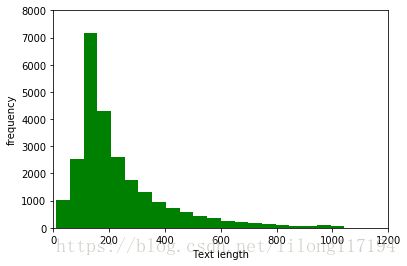
由图可以看出大部分的文本都在230之内,这里我的设置是250,也就是为训练样本中的每个样本提前开辟一个空间,用于存储样本向量。
(3) 得到索引矩阵
这是一个计算成本非常高的过程,这里使用的是提前运行保存的索引矩阵文件。当然了如果是自己的项目,那肯定要自己跑代码,等运行结果了。代码如下:
# 删除标点符号、括号、问号等,只留下字母数字字符
strip_special_chars = re.compile("[^A-Za-z0-9 ]+") # [^aeiou]:除了aeiou字母以外的所有字符

def cleanSentences(string):
    # replace是简单的替换
    string = string.lower().replace("
", " ")
    # re.sub是使用正则表达式来实现替换的功能
    return re.sub(strip_special_chars, "", string.lower())

# num_files:文件个数  25000
# max_seq_num:最大序列长度
# ids=15000 x 250的矩阵
max_seq_num = 250
ids = np.zeros((num_files, max_seq_num), dtype='int32')
file_count = 0

# 把文本中的正评价变成15000 x 250 的词ID矩阵
for pf in pos_files:
    with open(pf, "r", encoding='utf-8') as f:
        indexCounter = 0
        line = f.readline()
        cleanedLine = cleanSentences(line)
        split = cleanedLine.split()
        for word in split:
            try:
                #print('wordsList.index(word):',wordsList.index(word))
                #time.sleep(1)
                ids[file_count][indexCounter] = wordsList.index(word)
            except ValueError:
                ids[file_count][indexCounter] = 399999  # 未知的词
            indexCounter = indexCounter + 1
            # 这里如果是大于300长度的序列,那么就舍弃300以后的长度,所以就得到了15000x300的矩阵
            if indexCounter >= max_seq_num:
                break
        file_count = file_count + 1
        print('haha..')

# 把文本中的负评价变成15000 x 250 的词ID矩阵
for nf in neg_files:
    with open(nf, "r",encoding='utf-8') as f:
        indexCounter = 0
        line = f.readline()
        cleanedLine = cleanSentences(line)
        split = cleanedLine.split()
        for word in split:
              try:
                  ids[file_count][indexCounter] = wordsList.index(word)
              except ValueError:
                  ids[file_count][indexCounter] = 399999  # 未知的词语
              indexCounter = indexCounter + 1
              if indexCounter >= max_seq_num:
                  break
        file_count = file_count + 1
        print('oo..')
np.save('idsMatrix.npy', ids)
运行会得到全部电影训练集的索引矩阵,大小是25000 * 250 的矩阵
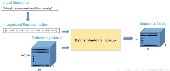
(4) 得到词向量:
对于一个新输入的句子或者文本,为了得到其词向量,我们可以使用 TensorFlow 的嵌入函数:tf.nn.embedding_lookup。这个函数有两个参数,一个是嵌入矩阵(在我们的情况下是词向量矩阵),另一个是每个词对应的索引。如下:
import tensorflow as tf
import numpy as np

maxSeqLength = 10
numDimensions = 300
wordsList = np.load('wordsList.npy')
print('载入word列表:',np.shape(wordsList))
wordsList = wordsList.tolist()
wordsList = [word.decode('UTF-8')  for word in wordsList]
wordVectors = np.load('wordVectors.npy')
print('载入文本向量:',wordVectors.shape)

firstSentence = np.zeros((maxSeqLength), dtype='int32')
firstSentence[0] = wordsList.index("i")
firstSentence[1] = wordsList.index("thought")
firstSentence[2] = wordsList.index("the")
firstSentence[3] = wordsList.index("movie")
firstSentence[4] = wordsList.index("was")
firstSentence[5] = wordsList.index("incredible")
firstSentence[6] = wordsList.index("and")
firstSentence[7] = wordsList.index("inspiring")
#firstSentence[8] and firstSentence[9] are going to be 0
print('firstSentence.shape:',firstSentence.shape)
print('firstSentence:',firstSentence)

with tf.Session() as sess:
    print(tf.nn.embedding_lookup(wordVectors,firstSentence).eval().shape)
运行结果:
输出数据是一个 10*50 的词矩阵,其中包括 10 个词,每个词的向量维度是 50,就是去找到这些词对应的向量,这里只是作为一个示例。
载入word列表: (400000,)
载入文本向量: (400000, 50)
firstSentence.shape: (10,)
firstSentence: [    41    804 201534   1005     15   7446      5  13767      0      0]
(10, 50)
数据管道如下:
(5) 批训练集函数:
def getTrainBatch():和def getTestBatch():
上面两个函数的功能就是构造训练集和测试集的每一批样本,可以发现有如下区间:
[1−11500]([11500−12500][12500−13500])[13500−25000] [ 1 − 11500 ] ( [ 11500 − 12500 ] [ 12500 − 13500 ] ) [ 13500 − 25000 ]
训练集中的每一批次正负样本都有,又能保证测试集里的样本没有在训练集中出现过。
(6) RNN Model

- 当确定好好两个占位符,一个用于数据输入,另一个用于标签数据。对于占位符,最重要的一点就是确定好维度。这里的标签占位符代表一组值,每一个值都为 [1,0] 或者 [0,1],这个取决于数据是正向的还是负向的。输入占位符,是一个整数化的索引数组。一旦,我们设置了我们的输入数据占位符,我们可以调用 tf.nn.embedding_lookup() 函数来得到我们的词向量。该函数最后将返回一个三维向量,第一个维度是批处理大小,第二个维度是句子长度,第三个维度是词向量长度。
- 堆栈 LSTM 网络是一个比较好的网络架构。也就是前一个LSTM 隐藏层的输出是下一个LSTM的输入。堆栈LSTM可以帮助模型记住更多的上下文信息,但是带来的弊端是训练参数会增加很多,模型的训练时间会很长,过拟合的几率也会增加。如果你想了解更多有关堆栈LSTM,可以查看TensorFlow的官方教程。
- dynamic RNN 函数的第一个输出可以被认为是最后的隐藏状态向量。这个向量将被重新确定维度,然后乘以最后的权重矩阵和一个偏置项来获得最终的输出值。
- 标准的交叉熵损失函数来作为损失值。对于优化器,我们选择 Adam,并且采用默认的学习率
(7) 超参数调整
选择合适的超参数来训练你的神经网络是至关重要的。你会发现你的训练损失值与你选择的优化器(Adam,Adadelta,SGD,等等),学习率和网络架构都有很大的关系。特别是在RNN和LSTM中,单元数量和词向量的大小都是重要因素。
- 学习率:RNN最难的一点就是它的训练非常困难,因为时间步骤很长。那么,学习率就变得非常重要了。如果我们将学习率设置的很大,那么学习曲线就会波动性很大,如果我们将学习率设置的很小,那么训练过程就会非常缓慢。根据经验,将学习率默认设置为 0.001 是一个比较好的开始。如果训练的非常缓慢,那么你可以适当的增大这个值,如果训练过程非常的不稳定,那么你可以适当的减小这个值。
- 优化器:这个在研究中没有一个一致的选择,但是 Adam 优化器被广泛的使用。
- LSTM单元的数量:这个值很大程度上取决于输入文本的平均长度。而更多的单元数量可以帮助模型存储更多的文本信息,当然模型的训练时间就会增加很多,并且计算成本会非常昂贵。
- 词向量维度:词向量的维度一般我们设置为50到300。维度越多意味着可以存储更多的单词信息,但是你需要付出的是更昂贵的计算成本。
(8) 训练过程
最好使用GPU进行训练,训练会用几个小时的时间,当然了,这要看硬件。。
上面也就是训练的过程,也可以同时在训练的同时,通过保存的模型来进行测试集的测试,但是我这里一直报错:
NotFoundError (see above for traceback): Key rnn/basic_lstm_cell/bias not found in checkpoint我的这个心啊。。。
改天再搞!!!
4. 语法使用
在使用中需要注意的地方有:
4.1 tensorflow的tf.argmax() 用法:
tf.argmax(input, dimension, name=None)
- dimension=0 按列找
- dimension=1 按行找
- tf.argmax()返回最大数值的下标
通常和tf.equal()一起使用,计算模型准确度,下面是使用:
import tensorflow as tf
a = tf.constant([1.,2.,3.,0.,9.,])
b = tf.constant([[1,2,3],[3,2,1],[4,5,6],[6,5,4]])
with tf.Session() as sess:
    print(sess.run(tf.argmax(a, 0)))
    print(sess.run(tf.argmax(b, 0)))
    print(sess.run(tf.argmax(b, 1)))
输出:
4
[3 2 2]
[2 0 2 0]
4.2 tf.gather用法
简单说就是获得相应下标的数据:
import tensorflow as tf

temp = tf.range(0,10)*10 + tf.constant(1,shape=[10])
temp2 = tf.gather(temp,[1,5,9])
with tf.Session() as sess:
    print (tf.range(0,10)*10)
    print (tf.constant(1,shape=[10]))
    print (sess.run(temp))
    print (sess.run(temp2))
输出:
Tensor("mul_1:0", shape=(10,), dtype=int32)
Tensor("Const_1:0", shape=(10,), dtype=int32)
[ 1 11 21 31 41 51 61 71 81 91]
[11 51 91]
注意:
macOS下的新建文件夹会自动生成一个.DS_Store的文件,会影响文件的读取,下面简单介绍下:
DS_Store 是给Finder用来存储这个文件夹的显示属性的:比如文件图标的摆放位置。删除以后的副作用就是这些信息的失去。
2 关闭.DS_Store的方法:
步骤一:删除所有隐藏.DS_store文件,打开命令行窗口
sudo find / -name ".DS_Store" -depth -exec rm {} \; 步骤二: 设置不再产生选项, 执行如下命令
defaults write com.apple.desktopservices DSDontWriteNetworkStores true 本文的代码是学习自:《pytho自然语言处理实战 核心技术与算法》
https://github.com/nlpinaction/learning-nlp/tree/master/chapter-8/sentiment-analysis
参考:https://www.aliyun.com/jiaocheng/517649.html