医学图像预处理（五） 器官与病灶的直方图

事情起因是：
用模型训练分割肝脏，效果还不错。但是训练分割肝脏肿瘤时，dice系数很低。由于已经经过ROI处理，和图像预处理过程，所以只可能是数据层面出现了问题。经过查看，发现很多ct图是即使用肉眼也无法分辨出肿瘤的。论文中给出的那种图片，肿瘤与肝脏对比度很高，但这种情况只是数据集中的少数。为了验证自己的想法，在LITS2017的数据集上，做出了130个病人对应的肝脏与肿瘤的hu直方图，发现果然如此。
但这样的话，论文里是如何获得那么好的结果的呢？？
（更新：2019-4-2，已完成肿瘤分割实验，写在博客：医学图像分割 基于深度学习的肝脏肿瘤分割 实战(二） ）

下面是代码，可以作为工具类使用：

import numpy as np
import SimpleITK as sitk
import matplotlib.pyplot as plt

onServer = False
if onServer:
    niiSegPath = './LITS17/seg/'
    niiImagePath = './LITS17/ct/'
else:
    niiSegPath = '~/LITS17/seg/'
    niiImagePath = '~/LITS17/ct/'
    
def getRangeImageDepth(image):
    z = np.any(image, axis=(1,2)) # z.shape:(depth,)
    #print("all index:",np.where(z)[0])
    if len(np.where(z)[0]) >0:
        startposition,endposition = np.where(z)[0][[0,-1]]
    else:
        startposition = endposition = 0
    
    return startposition, endposition
"""
会画出每个病人肿瘤区域最大切片的直方图
与汇总的直方图
"""
total_liver = []
total_tumor = []
colors = ['b','g']
for i in range(0, 131, 1):
    seg = sitk.ReadImage(niiSegPath+ "segmentation-" + str(i) + ".nii", sitk.sitkUInt8)
    segimg = sitk.GetArrayFromImage(seg)
    src = sitk.ReadImage(niiImagePath+"volume-" + str(i) + ".nii")
    srcimg = sitk.GetArrayFromImage(src)

    seg_liver = segimg.copy()
    seg_liver[seg_liver>0] = 1

    seg_tumorimage = segimg.copy()
    seg_tumorimage[segimg == 1] = 0
    seg_tumorimage[segimg == 2] = 1
    
    # 获取含有肿瘤切片的起、止位置
    start,end = getRangeImageDepth(seg_tumorimage)
    if start==0 and end == 0:
        print("continue")
        continue
    print("start:",start," end:",end)
    
    max_tumor=0 # 记录肿瘤的最大占比
    max_tumor_index = -1 # 记录最大肿瘤所在切片
    
    
    for j in range(start, end+1):
        if np.mean(seg_tumorimage[j]) > max_tumor:
            max_tumor = np.mean(seg_tumorimage[j])
            max_tumor_index = j
            
#        batch_image.append(srcimg[j,:,:])
#        batch_mask.append(seg_tumorimage[j,:,:])
    
    src_flatten = srcimg[max_tumor_index].flatten()
    liver_flatten = seg_liver[max_tumor_index].flatten()
    tumor_flatten = seg_tumorimage[max_tumor_index].flatten()
    
    liver = [] # liver hu value
    tumor = []
    for j in range(src_flatten.shape[0]):
        if liver_flatten[j]>0:
            liver.append(src_flatten[j])
        if tumor_flatten[j]>0:
            tumor.append(src_flatten[j])
            
    total_liver.append(liver)
    total_tumor.append(tumor)
    """    
    # 因为肝脏区域很多而肿瘤很少，所以画直方图使用相同的y-axis就会导致
    # 几乎看不到肿瘤的直方图
    plt.hist(flat_total_liver, color = "skyblue", bins=100, alpha=0.5, 	    label='liver hu')
    plt.hist(flat_total_tumor, color = "red", bins=100, alpha=0.5, label='tumor hu')
    plt.legend(loc='upper right')
    """
    fig, ax1 = plt.subplots()
    ax2 = ax1.twinx()
    ax1.hist([liver, tumor], bins=100,color=colors)
    n, bins, patches = ax1.hist([liver,tumor], bins=100)
    ax1.cla() #clear the axis
    
    #plots the histogram data
    width = (bins[1] - bins[0]) * 0.4
    bins_shifted = bins + width
    ax1.bar(bins[:-1], n[0], width, align='edge', color=colors[0])
    ax2.bar(bins_shifted[:-1], n[1], width, align='edge', color=colors[1])
    
    #finishes the plot
    ax1.set_ylabel("liver hu Count", color=colors[0])
    ax2.set_ylabel("tumor hu Count", color=colors[1])
    ax1.tick_params('y', colors=colors[0])
    ax2.tick_params('y', colors=colors[1])
    plt.tight_layout()
    plt.title("person[%d],slice[%d]"%(i,max_tumor_index))
    plt.savefig("LITS/person%d_slice%d.png"%(i,max_tumor_index))
    plt.clf() 
 
# 用来展平total_liver和total_tumor里面的值   
flat_total_liver = [item for sublist in total_liver for item in sublist]
flat_total_tumor = [item for sublist in total_tumor for item in sublist]
#plt.hist(flat_total_liver, color = "skyblue", bins=100, alpha=0.5, label='liver hu')
#plt.hist(flat_total_tumor, color = "red", bins=100, alpha=0.5, label='tumor hu')
#plt.legend(loc='upper right')
#plt.title("total hu")
#plt.savefig("LITS/total.png")
#plt.clf() 


fig, ax1 = plt.subplots()
ax2 = ax1.twinx()
ax1.hist([flat_total_liver, flat_total_tumor], bins=100,color=colors)
n, bins, patches = ax1.hist([flat_total_liver,flat_total_tumor], bins=100)
ax1.cla() #clear the axis

#plots the histogram data
width = (bins[1] - bins[0]) * 0.4
bins_shifted = bins + width
ax1.bar(bins[:-1], n[0], width, align='edge', color=colors[0])
ax2.bar(bins_shifted[:-1], n[1], width, align='edge', color=colors[1])

#finishes the plot
ax1.set_ylabel("liver hu Count", color=colors[0])
ax2.set_ylabel("tumor hu Count", color=colors[1])
ax1.tick_params('y', colors=colors[0])
ax2.tick_params('y', colors=colors[1])
plt.tight_layout()
plt.title("total")
plt.savefig("LITS/total.png")
plt.clf() 

论文里的图片通常是这样的：

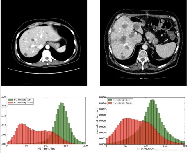
但实际上很多图是这样的（已经经过预处理）：

为了验证想法，作出原始hu值，发现确实如此，大约一半的病人肝脏与肿瘤的hu分布是对比度很强的，但另一半的情况是二者几乎重叠。（问了下学医的同学，说肝脏肿瘤分为很多种，连医生很多时候也无法通过ct判断，这时候就要做增强ct）下面是代码运行的部分结果展示