在深度神经网络中,输入特征通过从输入层开始前向传播 Forward propagation 来实现模型拟合,由于拟合的结果与给定的标签值通常存在一定的误差,而为了衡量这个误差,可以定义一个误差函数 Error / Loss function,此时网络的性能评价就被转化为一个函数优化问题:即如何通过一定的方法不断的调整作用在神经网络中不同层上的参数来降低误差函数的值,其中最重要的方法之一就是利用梯度下降 Gradient descent 来实现误差的反向传播 Backpropagation。理解这个过程是理解深度神经网络工作机理的核心,必须要反复推演以达到异常熟悉的程度,为此在这里做一个记录。文中所用代码对应的完整的 Jupyter Notebook 可以在我的 GitHub 上进行下载。
为了简化问题说明,这里用一个简单的 2 层神经网络来做一个演示,阐述梯度下降的原理和参数的更新过程。网络包含一个输入层,一个隐藏层,一个输出层,按照神经网络的命名规范在层数描述时忽略输入层,因此是一个 2 层的神经网络。请注意文中采用的图片来自 Udacity 深度学习纳米学位课程,版权归 Udacity 所有。
为了便于说明,先给出代码的实现过程,后续再进行分析:
import numpy as np

def sigmoid(x):
    # Use Sigmoid as the activation function
    return 1 / (1 + np.exp(-x))

x = np.array([0.5, 0.1, -0.2]) # here x is a rank 1 object
y = 0.6

learnrate = 0.5

weights_input_hidden = np.array([[0.5, -0.6],
                                 [0.1, -0.2],
                                 [0.1, 0.7]])

weights_hidden_output = np.array([0.1, -0.3]) # shape 2,

# Forward propagation
hidden_layer_input = np.dot(x, weights_input_hidden)
hidden_layer_output = sigmoid(hidden_layer_input) # shape 2,
#print(hidden_layer_output)

output_layer_input = np.dot(hidden_layer_output, weights_hidden_output)
output = sigmoid(output_layer_input)
#print(output) # a number

# Backwards propagation

# Calculate output error
error = y - output # a number, rank 0


# Calculate error term for output layer
output_error_term = error * output * (1 - output) # a number
#print(output_error_term)

# Calculate error term for hidden layer
hidden_error_term = output_error_term * weights_hidden_output *\
                    hidden_layer_output * (1 - hidden_layer_output) # shape 2,
#print(hidden_error_term)

# Calculate change in weights for hidden layer to output layer
weights_hidden_output += learnrate * output_error_term * hidden_layer_output # shape 2,

# Calculate change in weights for input layer to hidden layer
weights_input_hidden += learnrate * hidden_error_term * x[:, None]

#print('weights update for hidden layer to output layer:')
print(weights_hidden_output)
#print('weights update for input layer to hidden layer:')
print(weights_input_hidden)
Output:
[ 0.10804047 -0.29444082]
[[ 0.50017701 -0.60051118]
 [ 0.1000354  -0.20010224]
 [ 0.0999292   0.70020447]]
梯度下降 Gradient descent
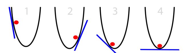
为了更加形象的给予说明,下图这个一元函数中假定其函数曲线代表一个误差函数,那么这个误差函数的最小值将在曲线的最底部取得,并且在此点斜率为 0。图中的红色小球所在的位置可以认为是函数随机取得某一自变量值时的误差值,假设我们为了通过算法实现小球可以自动其更新其位置来使得整个误差值可以最快的速度向误差缩减的方向进行,我们就需要为其设定某个特定的行进方向和行进速度。
从行进方向的角度,唯一可以利用的信息就是其所在点的斜率:
当斜率为正时,向左移动以减小斜率
当斜率为负时,向右移动以增加斜率
有了移动的方向以后,就需要考虑该以多大的速度进行移动:
在斜率绝对值较大时,表明小球离斜率为 0 的点较远,此时可以以较大的速度进行移动
当斜率绝对值较小时,表明小球离斜率为 0 的点较近,此时可以以较小的速度进行移动,以避免小球冲向对侧 overshoot
相应地,我们可以将移动的速度设置成斜率值本身或者斜率值的一个缩放值。
在一元函数中,函数的取值只跟随一个自变量的取值变化而变化,函数某点的斜率就是该点的导数值。但在多元函数中由于函数可以沿多个变量的方向变化,因此在函数的某一点上可以沿任意多个方向变化,因此就有了方向导数。为了描述其大小和方向,将方向导数定义为一个向量,而梯度的方向就是对应多元函数方向导数取值最大的方向,梯度的值就是方向导数的最大值。当多元函数上的点沿着其中一个自变量的方向变化,而其他自变量保持不变时,其函数取值的变化率称为偏导数。在实际的数学运算中,梯度的求解就是求多元函数针对各个自变量的偏导数。
我们将一元函数的经验予以推广,将多元误差函数的多个参数的更新方向参考该点的梯度的方向进行,并且更新的速度采用梯度的一个缩放值,所采用的缩放系数在深度学习的语境中就称为学习速率 Learning rate α 或 η。至此,我们就理解了利用梯度下降进行误差函数优化的原理。具体到深度学习中,在给定了输入特征和标签值之后,误差函数就由网络中散布在各个层中的权重参数决定,因此可以通过在随机初始化权重参数后计算误差值,在此基础上通过从误差向输出层再到隐藏层直至输入层逐层的分析各层的权重参数对于误差的贡献率,在此基础上对权重参数进行更新就可以实现误差函数的最小化。
误差的反向传播
有了以上的铺垫,我们就可以逐层地对代码的实现过程进行分析:
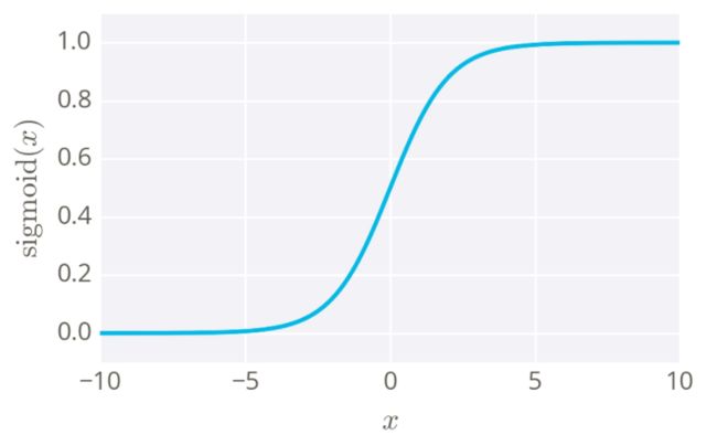
- 激活函数可以有多个选择,本例中选择的是 Sigmoid 函数,其函数定义为:σ(x) = 1 / (1 + e-x),这个函数的一个重要的特征是其取值范围为 (0, 1) ,因此结果可以看作一个概率,另一个重要特征是其导数为 σ(x)' = σ(x)(1 - σ(x)),这样在前向传播中已经计算过 σ(x) 的情况下,反向传播的梯度可以非常容易的计算。
def sigmoid(x):
    # Use Sigmoid as the activation function
    return 1 / (1 + np.exp(-x))
前向传播的计算过程比较直接,就是从输入开始在每一层通过点积计算输入与相应的权重参数的线性组合,再采用激活函数为模型添加非线性建模的能力:
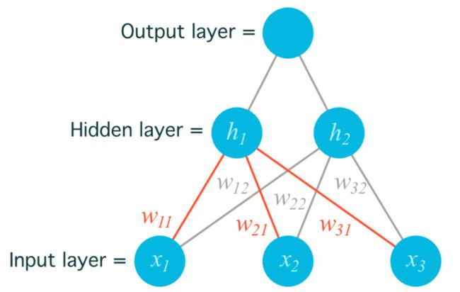
为了方便起见采用单个样本演示计算过程,输入层的每一个特征可以视作一个单元,所述样本涉及 3 个特征 x1,x2,x3,后续会对多个样本的情形进行说明
当一个隐藏层中包含多个单元,且输入以行向量形式与权重进行线性组合时,同一层不同单元中用到的权重参数会以列的形式被存储在参数矩阵中,记为
weights_input_hidden。参数矩阵中的元素通过 wij 的形式进行标记和索引,其中 i 为输入层的第 i 个单元,j 为隐藏层的第 j 个单元。对应每一个隐藏节点的线性运算部分为对所有输入特征的一个线性组合 hj,而隐藏层的输出则为对这个线性组合的激活 σ(hj) = σ(Σi wijxi),记为hidden_layer_output,本例中隐藏层单元的数量为 2,因此隐藏层权重矩阵的形状为 3 x 2输出层单元的数量为 1,因此输出层权重矩阵的形状为 2 x 1,记为
weights_hidden_output为了简化说明模型中忽略偏差值 b 的计算
x = np.array([0.5, 0.1, -0.2])
y = 0.6
learnrate = 0.5

weights_input_hidden = np.array([[0.5, -0.6],
                                 [0.1, -0.2],
                                 [0.1, 0.7]])

weights_hidden_output = np.array([0.1, -0.3])

# Forward propagation
hidden_layer_input = np.dot(x, weights_input_hidden)
hidden_layer_output = sigmoid(hidden_layer_input)

output_layer_input = np.dot(hidden_layer_output, weights_hidden_output)
output = sigmoid(output_layer_input)
衡量模型输出值和样本标签值差异的误差函数有多种选择方式,这里针对单个样本的误差 / 损失函数选择采用“误差的平方”这个函数:E = (y - ŷ)2 / 2,其中 y 为标签值,ŷ 为模型输出值。相关说明如下:
公式中除以 2 是为了约去求导产生的 2 的倍乘,使得最终误差计算的数学形式更简单
当实际应用中采用多个样本进行计算时,采用误差的平方可以进一步放大误差组成部分中贡献较大的项,进而可以在反向传播计算时,对于误差贡献较大的部分给予较大的惩罚 Penalty,可以更有效的减小误差
梯度的计算
注意这里的所有的梯度都是针对于各个层的权重参数来说的,因为对于训练来说,尽管输入用 X 表示,但实际上是已知的数值,网络中未知参数为权重参数。
在输出层,由于 :
- ŷ = σ(Σweights_hidden_output * hidden_layer_output)
则对于输出层权重参数的梯度有:
- ∂E / ∂whidden-output = ∂E / ∂ŷ * ∂ŷ / ∂whidden_output = -(y - ŷ) * layer_activation_derivative * hidden_layer_output
在输出层的前一个隐藏层,由于:
- ŷ = σ(Σweights_hidden_output * hidden_layer_output) = σ(Σweights_hidden_output * σ(Σweights_input_hidden * input_layer_output))
则对于隐藏层权重参数的梯度有:
- ∂E / ∂winput_hidden = ∂E / ∂ŷ * ∂ŷ / ∂h * ∂h / ∂winput_hidden = -(y - ŷ) * ŷ' * weights_hidden_output * hidden_layer_activation_derivative * input_layer_output
为了使的不同层的权重更新公式更加简洁统一,定义误差项:
- Error term δ = layer_error * layer_activation_derivative
即相应层输出的误差乘以该层的激活函数的导数。
在示例中由于激活函数为 Sigmoid 函数,则有:
输出层误差项 output_error_term = error * layer_activation_derivative
隐藏层误差项 hidden_error_term = output_error_term * weights_hidden_output * layer_activation_derivative
相应的权重更新的速度也即梯度 Δw 则可以表示成 learning_rate * δ * previous_layer_output 的形式,即
Δwoutput = learnrate * output_error_term * hidden_layer_output
Δwhidden = learnrate * hidden_error_term * input_layer_output
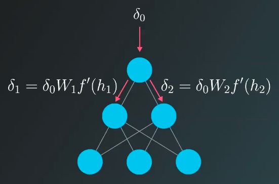
实际上,利用链式法则由输出向输入方向借助梯度来反向更新权重的过程,等同于将原有的神经网络反过来,以误差作为输入,使其在网络的各层中进行传播,并借此进一步了解误差在各层的分配情况。这也是 Backpropagation 这个名字的由来,此时可以更直观的解释为何隐藏层误差等于输出层误差项乘以两者之间的参数矩阵:
- hidden_error = np.dot(output_error_term, weights_hidden_output)
# Backwards propagation

# Calculate output error
error = y - output

# Calculate error term for output layer
output_error_term = error * output * (1 - output)

# Calculate error term for hidden layer
hidden_error_term = np.dot(output_error_term, weights_hidden_output) *\
                    hidden_layer_output * (1 - hidden_layer_output)

# Calculate change in weights for hidden layer to output layer
weights_hidden_output += learnrate * output_error_term * hidden_layer_output # shape 2,

# Calculate change in weights for input layer to hidden layer
weights_input_hidden += learnrate * hidden_error_term * x[:, None]

#print('weights update for hidden layer to output layer:')
print(weights_hidden_output)
#print('weights update for input layer to hidden layer:')
print(weights_input_hidden)
Output:
[ 0.10804047 -0.29444082]
[[ 0.50017701 -0.60051118]
 [ 0.1000354  -0.20010224]
 [ 0.0999292   0.70020447]]
最终的权重参数更新的大小也即原有的权重参数减去权重的梯度乘以学习速率:
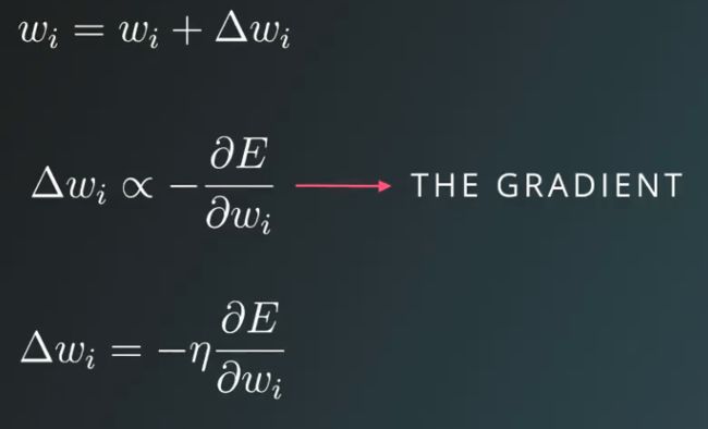
值得注意的是,图中 Δwi 之所以正比于负的 ∂E / ∂wi,是由于误差函数定义为 E = (y - ŷ)2 / 2,求导时会产生一个负号,进一步在参数更新中使用的是 wi = wi + Δwi。在有些例子中,如参考阅读中 Trask 的文章中误差定义为 E = (ŷ - y)2 / 2,则参数更新应该变为 wi = wi - Δwi。
多个样本的情形
当对网络提供多个样本时,可以将样本集的成本函数 Cost function 定义成误差平方和的 Sum of squared error,SSE:J = ΣL(ŷ(i), y(i)) = Σ(y - ŷ)2 / 2 或 Mean of squared error, MSE:J = ΣL(ŷ(i), y(i)) = Σ(y - ŷ)2 / 2m,其中 i = 1, 2, 3, ..., m,m 为样本的数量,在程序实现中只需在单个样本计算的基础上采用 for 循环遍历所有 m 个样本进行逐渐累加后即可,在 MSE 中再除以样本数量。
更高效的方式是采用 Numpy 将输入和标签向量化,同时计算一个批量中的各个训练样本在同一套权重参数下计算得到输出值,并采用前面的方法计算各个样本带来的权重更新值,最终用这个平均值来更新网络的参数。
import numpy as np

# use sigmoid as the activation function
def sigmoid(x):
    return 1 / (1 + np.exp(-x))

# This is a 2 layer neural network with 1 hidden layer, with 3 input features, 4 hidden layer units and 1 output unit.
X = np.array([[0, 0, 1],
            [0, 1, 1],
            [1, 0, 1],
            [1, 1, 1]])

y = np.array([[0],
            [1],
            [1],
            [0]])

n_features = X.shape[1]

# set the learing rate to 10 here
alpha = 10

#seeds the random module so the results are the same for debugging convenience
np.random.seed(32)

# randomly initialize our weights with mean 0
weights_input_hidden = np.random.normal(scale= 1 / n_features**0.5, size=(3, 4))
weights_hidden_output = np.random.normal(scale = 1 / n_features**0.5, size=(4, 1))

print("Initial weights: ")
print(weights_input_hidden)
print(weights_hidden_output)

# train for 100 times with 4 inputs together
for j in range(100):

    # Feed forward through hidden layer and output layer
    hidden_layer_output = sigmoid(np.dot(X, weights_input_hidden)) # shape: 4, 4
    final_output = sigmoid(np.dot(hidden_layer_output, weights_hidden_output)) # shape: 4, 1

    # the difinition of error actually determine the positive or negative addition of the weights
    final_output_error = y - final_output # shape: 4, 1

    # final output error term equals output error times the derivatives of output layer's activation fuction
    final_output_error_term = final_output_error * final_output * (1 - final_output) # shape 4, 1

    # how much did each hidden layer value contribute to the output layer error (according to the weights)?
    hidden_layer_output_error = final_output_error_term.dot(weights_hidden_output.T) # shape: 4, 1 * 1, 4
    hidden_layer_output_error_term = hidden_layer_output_error * hidden_layer_output * (1 - hidden_layer_output) # shape 4, 4

    # weights change for each epoch
    weights_hidden_output_difference = np.dot(hidden_layer_output.T, final_output_error_term) # shape 4, 1 = 4, 4 * 4, 1
    weights_input_hidden_difference = np.dot(X.T, hidden_layer_output_error_term) # shape 3, 4 = 3, 4 * 4, 4

    # update the weights with averaged difference derived by all inputs
    weights_hidden_output += alpha * weights_hidden_output_difference / n_features
    weights_input_hidden += alpha * weights_input_hidden_difference / n_features

    if j > 0 and j % 20 == 0:
        print("Error after "+ str(j) +" iterations: " + str(np.mean(final_output_error**2)))
        print("Weights update after every 20 epoch: ")
        print(weights_input_hidden)
        print(weights_hidden_output)
Output:
Initial weights:
[[-0.20143431  0.56794144  0.33539595  0.04057874]
 [ 0.4489087   0.33599404  0.84973866  0.960238  ]
 [-0.15079068 -0.39760774 -0.40121413  1.12030401]]
[[ 1.04235695]
 [ 0.26345293]
 [-0.33186789]
 [ 0.06592214]]
Error after 20 iterations: 0.249671646691
Weights update after every 20 epoch:
[[-0.31186521  0.57647642  0.21399002 -0.13309149]
 [ 0.42749989  0.33908914  0.7814787   0.96151458]
 [-0.3479972  -0.40109341 -0.480883    1.11669635]]
[[ 0.87226058]
 [ 0.13100723]
 [-0.46314094]
 [-0.25683172]]
Error after 40 iterations: 0.248555608688
Weights update after every 20 epoch:
[[-0.45821546  0.61137029  0.1644987  -0.37881868]
 [ 0.49678079  0.36928896  0.74287451  1.00909503]
 [-0.47135973 -0.36300227 -0.55002109  1.10811792]]
[[ 0.94413674]
 [ 0.22826295]
 [-0.41109329]
 [-0.38283076]]
Error after 60 iterations: 0.243826210867
Weights update after every 20 epoch:
[[-0.7921686   0.70025013  0.14881824 -0.80393464]
 [ 0.69027893  0.45415457  0.72157744  1.20239422]
 [-0.67376173 -0.26738321 -0.6111616   1.09236471]]
[[ 1.1684149 ]
 [ 0.43940071]
 [-0.31528762]
 [-0.68466592]]
Error after 80 iterations: 0.208572028959
Weights update after every 20 epoch:
[[-1.72609207  1.00284109  0.15137427 -1.62484956]
 [ 1.38439873  0.78482729  0.71511052  1.93066983]
 [-1.09006185  0.00364683 -0.66122388  1.20971745]]
[[ 1.95281262]
 [ 0.93200691]
 [-0.16363967]
 [-1.5312133 ]]
最后有一点需要注意的就是,第一个例子由于采用单一样本,因此在 Udacity 的课程里建议使用的是 np.array([1, 3, 4]) 这种形式的数据结构,这在我看来是一个非常不好的建议。事实上在 Andrew Ng 的课堂上强烈建议大家不要采用这种结构,因为很可能带来意想不到的隐形 bugs,实际上我也遇到了这个问题。当然这也可以理解为个人喜好,我个人倾向于 Andrew 的方法,具体原因分析请见 捡个七 - rank 1 array 对于这个问题的分析。
参考阅读
Andrew Trask - A Neural Network in 13 lines of Python - Part 1
Andrew Trask - A Neural Network in 13 lines of Python - Part 2