随机森林分析在宏基因组数据分析中还是蛮常见的,所以这里整理一个常规的分析案例
1 | 数据准备
1.1 菌群数据

图一 菌群数据-OTU
1.2 样品信息数据
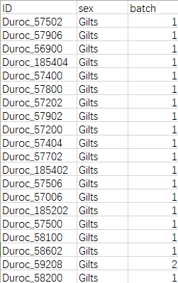
图二 样品信息数据
2 | 直接贴代码
#For windows system#
##ramdomforest.crossvalidation.r##
rm(list=ls())
# loading packages if necessary
library(randomForest)
library(ggplot2)
library(caret)
library(tidyverse)
# setting your working directory
setwd("E:\\F6_castrate_analysis\\total\\Duroc 16S\\fsm\\OTU\\稀疏后的OTU表")
set.seed(123)
## group male before and after castration

# loading Your datasets
dat1 <- read.table("fsm_otu_profile.csv",header=T,sep=',',row.names = 1)
conf <- read.table("fsm_metadata.csv",header=T,sep=',',row.names = 1)
#calculate the relative abundance of dat1
#dat1 <- sweep(dat1,2,colSums(dat1),'/')*100
dat1 <- log10(dat1 + 1)/log10(max(dat1))
cN.prof <- colnames(dat1)
#cN.prof <- sub("X","",cN.prof)
rN.conf <- rownames(conf)
gid <- intersect(cN.prof ,rN.conf) #求A和B的交集,根据样品名
dat1 <- dat1[,pmatch(gid,cN.prof)] # pmatch部分匹配
conf <- conf[pmatch(gid,rN.conf),]
dat2<-dat1[,conf$sex=="Gilts" | conf$sex=="Entire boars"]
conf2<-conf[conf$sex=="Gilts" | conf$sex=="Entire boars",]
conf2$sex=as.factor(as.character(conf2$sex))
outcome=conf2$sex
outcome<-sub("Gilts","0",outcome)
outcome<-sub("Entire boars","1",outcome)
outcome<-as.factor(outcome)
dat<-dat2
X <- as.data.frame(t(dat))
X$outcome = outcome

# 随机1-2有放回抽样293次,概率分别为0.67和0.33,用于获取训练集
ind = sample(2,nrow(X),replace=TRUE, prob=c(0.67,0.33))
# 2/3作预测建模
ind.train <- X[ind == 1,]
ind.test <- X[ind == 2,]

set.seed(123)

# 1.在随机森林算法的函数randomForest()中有两个非常重要的参数,
# 而这两个参数又将影响模型的准确性
# 2.它们分别是mtry和ntree。一般对mtry的选择是逐一尝试,直到找
# 到比较理想的值,ntree的选择可通过图形大致判断模型内误差稳定时的值。

# 选取randomforest函数中的mtry节点值,一般可默认,mtry指定节点中用于二叉树的变量个数
# 默认情况下为数据集变量个数的二次方根(分类模型)或三分之一(预测模型)

n <- length(names(ind.train))
set.seed(100)
errRate <- NULL
for(i in 1:(n-1)){
  mtry_fit <- randomForest(outcome ~ ., data = ind.train, mtry = i)
  err <- mean(mtry_fit$err.rate)
  errRate[i] <- err
}
# 选择平均误差最小的mtry
m <- which.min(errRate)
# m为221

# 之后选择ntree值,ntree指定随机森林所包含的决策树数目,默认为500,
set.seed(100)
ntree_fit <- randomForest(outcome ~ ., data = ind.train, mtry = 221, ntree = 1000)
plot(ntree_fit) # ntree到600以后就基本不变

# 根据以上结果,默认情况下的mtry效果更好,所以以mtry=18,ntree=600为参数构建随机森林模型。
rf.train <- randomForest(outcome ~ ., data = ind.train, mtry = 18,
                         importance = TRUE,proximity=TRUE,ntree = 600)
print(rf.train)
#summary(rf)
#' 交叉验证选择features
# set.seed(123)
#' rfcv是随机森林交叉验证函数:Random Forest Cross Validation
# result <- rfcv(X[,-ncol(X)],X$outcome,cv.fold = 10)
# result$error.cv #' 查看错误率表,21时错误率最低,为最佳模型
#' 绘制验证结果
# with(result,plot(n.var,error.cv,log="x",type = "o",lwd=2))
# 使用replicate进行多次交叉验证,可选
result <- replicate(5, rfcv(ind.train[,-ncol(ind.train)],ind.train$outcome,cv.fold = 20), simplify=FALSE)
error.cv <- sapply(result, "[[", "error.cv")
error.cv <- cbind(rowMeans(error.cv),error.cv)
n.var = rownames(error.cv) %>% as.numeric()
error.cv = error.cv[,2:6]
colnames(error.cv) = paste('err',1:5,sep='.')
err.mean = apply(error.cv,1,mean)
allerr = data.frame(num=n.var,err.mean=err.mean,error.cv)
# number of features selected
optimal = 164


# 表格输出
write.table(allerr, file = "family_rfcv.txt", sep = "\t", quote = F, row.names = T, col.names = T)
# the pre-setted parameters used for ploting afterwards
main_theme = theme(panel.background=element_blank(),
                   panel.grid=element_blank(),
                   axis.line.x=element_line(size=.5, colour="black"),
                   axis.line.y=element_line(size=.5, colour="black"),
                   axis.ticks=element_line(color="black"),
                   axis.text=element_text(color="black", size=7),
                   legend.position="right",
                   legend.background=element_blank(),
                   legend.key=element_blank(),
                   legend.text= element_text(size=7),
                   text=element_text(family="sans", size=7))

p = ggplot() +
  geom_line(aes(x = allerr$num, y = allerr$err.1), colour = 'grey') +
  geom_line(aes(x = allerr$num, y = allerr$err.2), colour = 'grey') +
  geom_line(aes(x = allerr$num, y = allerr$err.3), colour = 'grey') +
  geom_line(aes(x = allerr$num, y = allerr$err.4), colour = 'grey') +
  geom_line(aes(x = allerr$num, y = allerr$err.5), colour = 'grey') +
  geom_line(aes(x = allerr$num, y = allerr$err.mean), colour = 'black') +
  geom_vline(xintercept = optimal, colour='black', lwd=0.36, linetype="dashed") +
  #  geom_hline(yintercept = min(allerr$err.mean), colour='black', lwd=0.36, linetype="dashed") +
  coord_trans(x = "log2") +
  scale_x_continuous(breaks = c(1, 3, 5, 10, 20, 40, 60, 100, 200, 300)) + # , max(allerr$num)
  labs(title=paste('Training set (n = ', dim(dat)[2],')', sep = ''),
       x='Number of OTUs ', y='Cross-validation error rate') +
  annotate("text", x = optimal, y = max(allerr$err.mean), label=paste("optimal = ", optimal, sep="")) +
  main_theme
ggsave(p, file = "duroc_otu_rfcv.pdf", width = 89, height = 50, unit = 'mm')
p


###--------------------------------------######
###----       将最佳的那164个OTUs         ######

imp <- as.data.frame(rf.train$importance)
# 随机森林中的特征重要性表示在该特征上拆分的所有节点的基尼不纯度减少的总和
# 减少的越多,说明该特征在分类过程中起的作用越大。
imp <- imp[order(imp[,1],decreasing = T),]
#head(imp)
#' 输出重要性排序的表格
#write.table(imp,file = "importance_class_20180719.txt",quote = F,sep = '\t',row.names = T,col.names = T)
#' 简单可视化
varImpPlot(rf,main = "Top 164-feature OTU importance",n.var = 164,bg=par("bg"),
           color = par("fg"),gcolor=par("fg"),lcolor="gray")

#' 美化feature贡献度柱状图
#' 分析选择top5效果最好
imp = head(imp, n=164)
write.table(imp,file = "importance_class_selected.txt",quote = F,sep = '\t',row.names = T,col.names = T)
#' 反向排序X轴,让柱状图从上往下画
imp = imp[order(imp[,3],decreasing = F),]
imp$name <- rownames(imp)
imp$name <- factor(imp$name,levels = imp$name)
OTU_attribution <- read.table("OTU_phylum.csv",header = T,sep = ",",check.names = F)
rownames(OTU_attribution) <- OTU_attribution$OTUID
OTU_attribution <- OTU_attribution[rownames(imp),]
imp$phylum <- OTU_attribution$phylum
imp2 <- imp
rownames(imp2) <- paste(rownames(imp2),OTU_attribution$class,sep = " ")
imp2$name <- rownames(imp2)
imp2$name <- factor(imp2$name,levels = imp2$name)
#' load ggplot2 package
library(ggplot2)
p <- ggplot(imp2,aes(x=name,y=MeanDecreaseAccuracy,fill=phylum)) +
  geom_bar(stat = "identity") + coord_flip()
p <- p+theme_bw()
p <- p+theme(legend.position = c(0.75,0.15))
p <- p + theme(plot.background=element_blank(),panel.background=element_blank())
p <- p + theme(axis.text.x=element_text(face="bold",color="black",size=14),
               axis.text.y=element_text(face = "bold",color="black",size = 14),
               axis.title.y=element_text(size = 16,face = "bold"),axis.title.x=element_text(size = 16))
p <- p + scale_fill_manual(values=c("red2", "blue4","yellow2"))
p + theme(legend.background = element_blank())
p <- p + theme(
  legend.key.height=unit(0.8,"cm"),
  legend.key.width=unit(0.8,"cm"),
  legend.text=element_text(lineheight=0.8,face="bold",size=16),
  legend.title=element_text(size=18,face = "bold"))
p <- p+labs(x="OTU rank")
ggsave(paste("rf_imp_feature" , ".tiff", sep=""), p, width = 10, height = 6)

###---------------------------------###
###---     热图展示其丰度      -----###
# ' 筛选82个feature 展示
sub_abu = X[,rownames(imp)]
#' transposition the data
sub_abu <- as.data.frame(t(sub_abu))
#' table(X$outcome)
#'  0   1
#' 108 185
#sub_abu$class <- X$outcome
#sub_abu$class <- sub("0","Gilts",sub_abu$class)
#sub_abu$class <- sub("1","Entire_boars",sub_abu$class)
sub_abu_matrix <- as.matrix(sub_abu)
library(pheatmap)
annotation_col <- data.frame(Group=factor(rep(c("Gilts","Entire_boars"),c(108,185))))
rownames(annotation_col) <- colnames(sub_abu_matrix)
ann_colors <- list(Group=c(Gilts="#4DAF4A",Entire_boars="#984EA3"))
#plot.new()
tiff("OTU_rf_pheatmap.tiff",width = 6000,height = 1200,res = 300)
pheatmap(sub_abu_matrix,treeheight_col = 20,annotation_colors = ann_colors,cluster_cols = FALSE,
         cluster_rows = FALSE,show_colnames = FALSE,annotation_col=annotation_col,
         gaps_col = c(108,108),border_color = "NA",cellwidth = 4.3,cellheight = 20)
dev.off()

#' 用选择好的164个OTU重新构建randomforest模型
ind.train2 <- cbind(ind.train[,rownames(imp)], ind.train$outcome)
names(ind.train2)[ncol(ind.train2)] <- "class"
rf.train2 <- randomForest(class ~ ., data = ind.train2, importance = TRUE,
                          proximity = TRUE, ntree = )

# 预测响应变量
ind.train2$predicted.response <- predict(rf.train2, ind.train2)

# confusionMatrix function from caret package can be used for
# creating confusion matrix based on actual response
# variable and predicted value(构建混淆矩阵建立真实响应变量和预测响应变量值)
confusionMatrix(data=ind.train2$predicted.response, reference=ind.train2$class)

# 测试训练集
ind.test <- cbind(ind.test[,rownames(imp)], ind.test$outcome)
names(ind.test)[ncol(ind.test)] <- "class"
# 预测训练集的响应变量
ind.test$predicted.reponse <- predict(rf.train2, ind.test)
confusionMatrix(data=ind.test$predicted.reponse, reference=ind.test$class)

#rf.test <- randomForest(class ~ ., data = ind.test,
#                        importance = TRUE,proximity=TRUE,ntree = 1000)
#rf.test.pre <- predict(rf.test,type="prob")
#p.train<-rf.test.pre[,2]
########ROC in train######
library(pROC)
predicted.reponse <- predict(rf.train2, ind.test, type = "prob")
roc(ind.test$class,predicted.reponse[,2])
###################
roc1 <- roc(ind.test$class,
            predicted.reponse[,2],
            partial.auc.correct=TRUE,
            ci=TRUE, boot.n=100, ci.alpha=0.9, stratified=FALSE,
            plot=F, auc.polygon=TRUE, max.auc.polygon=TRUE, grid=TRUE)
#####################
tiff("fsm_variable_pROC.tiff",width=2200,height=1800,res=300)
roc1 <- roc(ind.test$class, predicted.reponse[,2],
            ci=TRUE, boot.n=100, ci.alpha=0.9, stratified=FALSE,font=2, font.lab=2,
            plot=TRUE, percent=roc1$percent,col="#F781BF",cex.lab=1.2, cex.axis=1.2,cex.main=1.5)
plot(roc1,col="black",add=T)
legend("bottomright",cex=1.4,c(paste("AUC=",round(roc1$ci[2],2),"%"),
                               paste("95% CI:",round(roc1$ci[1],2),"%-",round(roc1$ci[3],2),"%")))
dev.off()
3 | 结果展示
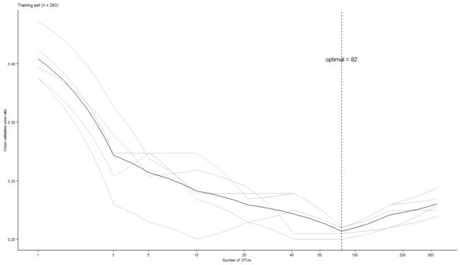
图三 选择了82个OTU,使得模型的错误率最低
参考
- https://zhuanlan.zhihu.com/p/51165358
- https://www.r-bloggers.com/lang/chinese/1077
- https://www.cnblogs.com/nxld/p/6374945.html
- https://zhuanlan.zhihu.com/p/24416833