5.logistic 回归模型

大纲

1. idea --- 理解logistic 回归原理

2. look --- 训练权值

3. code --- python

---

得先明确一下，这篇文章炒鸡枯燥的说。非要看的话，得听我解释一下这篇文章的思路，要不会很凌乱的。

• 首先是对logistic模型的核心公式解释
• 然后带入以前的Perceptron计算模型中，来体现logistic模型的作用
• 解释模型中出现的概念和意义
• 推导模型中公式
• 训练算法的原理（极大似然法）
• 用算法包实现一下看看
• 都看到最后一条了开始看吧~

---

logistic 模型概述

输出Y：{0,1}发生了事件->1，未发生事件->0
输入X1，X2...Xm
P表示m个输入作用下，事件发生（y=1）的概率
是一个由条件概率分布表示的2元分类模型

事件发生概率

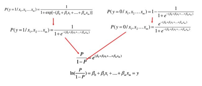
logistic逻辑回归模型就是，将输入x和权值w的线性函数表示为输出Y=1的概率（概念解释和公式推导在后面）

Paste_Image.png

优势（odds）

事件发生的概率和不发生的概率比，即 P/(1-P)

优势比（odds ratio：OR）

衡量某个特征的两个不同取值（C0，C1），对于结果的影响大小。OR>1事件发生概率大，是危险因素，OR<1事件发生概率小，是保护因素，OR=1该因素与事件发生无关

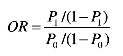
OR：odds ratio

logit变换

事件发生于事件未发生之比的自然对数，叫做P的logit变换，logit（P）

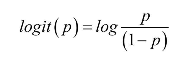
logit变换

logistic 函数

函数图像为一个S形函数：sigmoid function

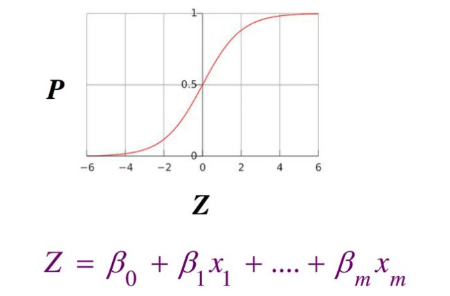
S形函数

利用极大似然发拟合最佳参数

似然函数可以理解为条件概率的逆反
已知事件Y发生，来估计参数x·w的最合理的可能，即计算能预测事件Y的最佳x·w的值.

带入logistic模型得以下公式

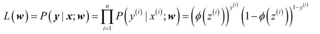
似然函数

为了简单求得最大值，我们使用对数似然函数

对数似然函数

转换成代价函数

我们用一个梯度上升的方法来使对数似然函数最大化，我们将对数似然函数重写成代价函数的模式，然后利用梯度下降的方法求代价最小对应的权值

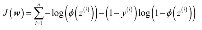
代价函数，对数似然函数重写而来

整理成更易于阅读和理解的形式

代价函数

在预测y=0和y=1的情况下，如下图公式所示

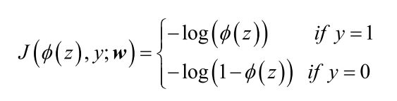
Paste_Image.png

代价函数如图，预测准确的情况下误差趋于0，预测错误就会趋于无穷

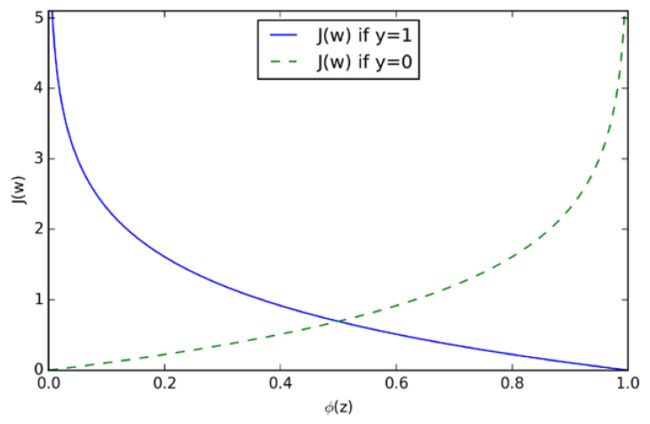
代价函数图形

Code Time

绘制S函数

# encoding:utf-8
__author__ = 'Matter'

import matplotlib.pyplot as plt
import numpy as np

def sigmoid(z):
    return 1.0 / (1.0+np.exp(-z))

z = np.arange(-5,5,0.05)
phi_z = sigmoid(z)

plt.plot(z,phi_z)
plt.axvline(0.0,color='k')
plt.ylim(-0.1,1.1)

plt.yticks([0.0,0.5,1.0])
ax = plt.gca()
ax.yaxis.grid(True)

plt.show()

S型函数

Logistic 逻辑回归函数

# encoding:utf-8
__author__ = 'M'
# 读取数据
from sklearn import datasets
import numpy as np
iris = datasets.load_iris()
X = iris.data[:,[2,3]]
y = iris.target

# 训练数据和测试数据分为7:3
from sklearn.cross_validation import train_test_split
x_train,x_test,y_train,y_test =train_test_split(X,y,test_size=0.3,random_state=0)

# 标准化数据
from sklearn.preprocessing import StandardScaler
sc = StandardScaler()
sc.fit(x_train)
x_train_std = sc.transform(x_train)
x_test_std = sc.transform(x_test)

# 绘制决策边界
from matplotlib.colors import ListedColormap
import matplotlib.pyplot as plt
import warnings

def versiontuple(v):
    return tuple(map(int, (v.split("."))))

def plot_decision_regions(X,y,classifier,test_idx=None,resolution=0.02):
    # 设置标记点和颜色
    markers = ('s','x','o','^','v')
    colors = ('red', 'blue', 'lightgreen', 'gray', 'cyan')
    cmap = ListedColormap(colors[:len(np.unique(y))])

    # 绘制决策面
    x1_min, x1_max = X[:, 0].min() - 1, X[:, 0].max() + 1
    x2_min, x2_max = X[:, 1].min() - 1, X[:, 1].max() + 1
    xx1, xx2 = np.meshgrid(np.arange(x1_min, x1_max, resolution),
                         np.arange(x2_min, x2_max, resolution))
    Z = classifier.predict(np.array([xx1.ravel(), xx2.ravel()]).T)
    Z = Z.reshape(xx1.shape)
    plt.contourf(xx1, xx2, Z, alpha=0.4, cmap=cmap)
    plt.xlim(xx1.min(), xx1.max())
    plt.ylim(xx2.min(), xx2.max())

    for idx, cl in enumerate(np.unique(y)):
        plt.scatter(x=X[y == cl, 0], y=X[y == cl, 1],
                    alpha=0.8, c=cmap(idx),
                    marker=markers[idx], label=cl)

    # 高粱所有的数据点
    if test_idx:
        # 绘制所有数据点
        if not versiontuple(np.__version__) >= versiontuple('1.9.0'):
            X_test, y_test = X[list(test_idx), :], y[list(test_idx)]
            warnings.warn('Please update to NumPy 1.9.0 or newer')
        else:
            X_test, y_test = X[test_idx, :], y[test_idx]
        plt.scatter(X_test[:, 0], X_test[:, 1], c='',
                alpha=1.0, linewidth=1, marker='o',
                s=55, label='test set')

# 应用Logistics回归模型
from sklearn.linear_model import LogisticRegression
lr = LogisticRegression(C=1000.0,random_state=0)
lr.fit(x_train_std,y_train)

X_combined_std = np.vstack((x_train_std, x_test_std))
y_combined = np.hstack((y_train, y_test))
plot_decision_regions(X_combined_std, y_combined,
                      classifier=lr, test_idx=range(105,150))
plt.xlabel('petal length [standardized]')
plt.ylabel('petal width [standardized]')
plt.legend(loc='upper left')
plt.tight_layout()
plt.show()

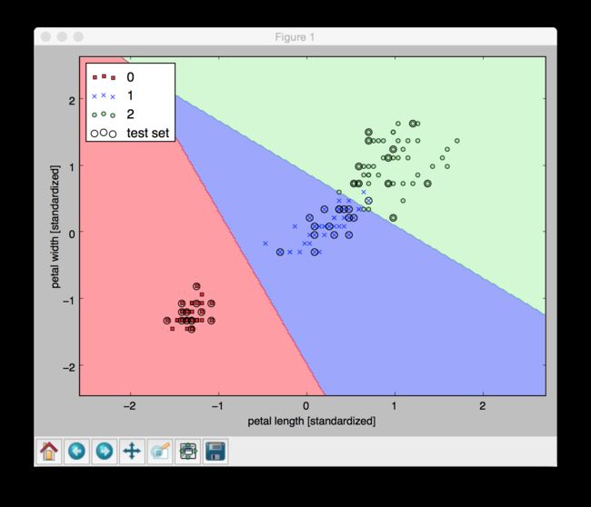
Logistics 回归函数分类结果