单细胞转录组||Seurat新版教程:Guided Clustering Tutorial

Seurat - Guided Clustering Tutorial

Seurat，一个单细胞数据分析工具箱

pipeline流程图

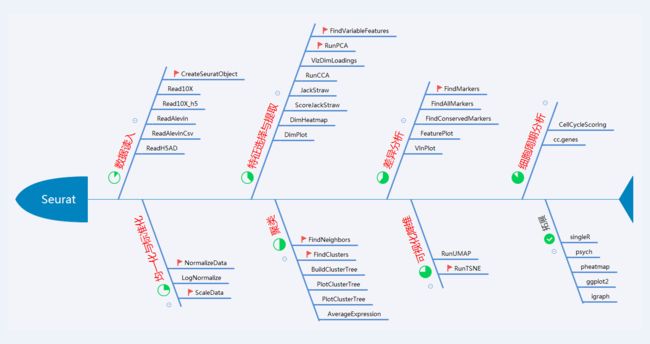
十大函数

支撑这个鱼骨架的是是下面的十个函数，细心的读者也许已经发现，大师已经插上了小红旗。在Seurat v2到v3的过程中，其实是有函数名变化的，当然最主要的我认为是参数中gene到features的变化，这也看出Seurat强烈的求生欲——既然单细胞不止做转录组那我也就不能单纯地叫做gene了，所有表征单细胞的features均可以用我Seurat来分析了。另外，相对于features而言gene只不过是一个实例而已。所以在升级Seurat的时候一个关键的地方就是函数名以及参数的更改。至于新的功能和算法其实并不多，如果用不到Seurat v3的新功能（如UMAP降维）其实不升级到v3做单细胞转录组是完全没问题的。

据不完全统计Seurat包大约有130多个函数，我们有必要问号一遍吗？不必要，当你有需求的时候去查就好了，但是人类很多时候并不知道自己需要的是什么，所以我建议还是把他的函数说明手册拿出来浏览一遍，至少把目录看一遍，大概知道他能做什么。

> library(Seurat)
> packageVersion("Seurat")
[1] ‘3.0.1’

pbmc.counts <- Read10X(data.dir = "D:\\Users\\Administrator\\Desktop\\RStudio\\single_cell\\filtered_gene_bc_matrices\\hg19")
pbmc <- CreateSeuratObject(counts = pbmc.counts)
pbmc <- NormalizeData(object = pbmc)
pbmc <- FindVariableFeatures(object = pbmc)
pbmc <- ScaleData(object = pbmc)
pbmc <- RunPCA(object = pbmc)
pbmc <- FindNeighbors(object = pbmc)
pbmc <- FindClusters(object = pbmc)
pbmc <- RunTSNE(object = pbmc)

数据读入

library(Seurat)
packageVersion("Seurat")
[1] ‘3.0.1’
# https://satijalab.org/seurat/mca.html
library(dplyr)
library(ggsci)#我想改变一下配色

学习一个R包当然是把他的标准流程走一遍了，下载它的官网数据放在我的电脑上。

# Load the PBMC dataset
list.files("D:\\Users\\Administrator\\Desktop\\RStudio\\single_cell\\filtered_gene_bc_matrices\\hg19")

[1] "barcodes.tsv"       "genes.tsv"          "matrix.mtx"    
?Read10X
## Not run: 
# For output from CellRanger < 3.0
data_dir <- 'path/to/data/directory'
list.files(data_dir) # Should show barcodes.tsv, genes.tsv, and matrix.mtx
expression_matrix <- Read10X(data.dir = data_dir)
seurat_object = CreateSeuratObject(counts = expression_matrix)

# For output from CellRanger >= 3.0 with multiple data types
data_dir <- 'path/to/data/directory'
list.files(data_dir) # Should show barcodes.tsv.gz, features.tsv.gz, and matrix.mtx.gz
data <- Read10X(data.dir = data_dir)
seurat_object = CreateSeuratObject(counts = data$`Gene Expression`)
seurat_object[['Protein']] = CreateAssayObject(counts = data$`Antibody Capture`)

也就是说Seurat可以直接用Read10X函数读取cellrangerV2 和V3的数据了，省去了不少麻烦是不是？！

创建Seurat对象。

pbmc.data <- Read10X(data.dir = "D:\\Users\\Administrator\\Desktop\\RStudio\\single_cell\\filtered_gene_bc_matrices\\hg19")
# Initialize the Seurat object with the raw (non-normalized data).
?CreateSeuratObject
pbmc <- CreateSeuratObject(counts = pbmc.data, project = "pbmc3k", min.cells = 3, min.features = 200)
> pbmc

An object of class Seurat 
13714 features across 2700 samples within 1 assay 
Active assay: RNA (13714 features)

如果不是10X的技术,如是BD流程，得到表达矩阵后,也是可以用Seurat分析的。需要注意的是矩阵要是要求矩阵行为基因，列为细胞编号。

library(Matrix) 
matrix = read.delim(matrix.path, header = T, stringsAsFactors = FALSE) 
pbmc <- CreateSeuratObject(counts = matrix, project = "project name", min.cells = 3, min.features = 200) # 参数自己写的
> pbmc # 检查一下是否读对了。

创建完其实是有两个S4类数据集的，一个是Seurat对象一个是bgCMatrix，要知道每个对象中存储的是什么数据，可以通过或者 $来提取查看：

线粒体细胞和红细胞比例。

# The [[ operator can add columns to object metadata. This is a great place to stash QC stats
pbmc[["percent.mt"]] <- PercentageFeatureSet(pbmc, pattern = "^MT-")
?PercentageFeatureSet
HB.genes_total <- c("HBA1","HBA2","HBB","HBD","HBE1","HBG1","HBG2","HBM","HBQ1","HBZ") # 人类血液常见红细胞基因
HB_m <- match(HB.genes_total,rownames(pbmc@assays$RNA))

HB.genes <- rownames(pbmc@assays$RNA)[HB_m]
HB.genes <- HB.genes[!is.na(HB.genes)]
pbmc[["percent.HB"]]<-PercentageFeatureSet(pbmc,features=HB.genes)

# write  nGene_nUMI_mito_HB
head([email protected])[,c(2,3,4,5)]

               nCount_RNA nFeature_RNA percent.mt percent.HB
AAACATACAACCAC       2419          779  3.0177759          0
AAACATTGAGCTAC       4903         1352  3.7935958          0
AAACATTGATCAGC       3147         1129  0.8897363          0
AAACCGTGCTTCCG       2639          960  1.7430845          0
AAACCGTGTATGCG        980          521  1.2244898          0
AAACGCACTGGTAC       2163          781  1.6643551          0

Feature、count、线粒体基因、红细胞基因占比可视化。

# Visualize QC metrics as a violin plot
VlnPlot(pbmc, features = c("nFeature_RNA", "nCount_RNA", "percent.mt","percent.HB"), ncol = 4)#+scale_color_npg() 不起作用
#p1_aaas = p1 + scale_color_aaas()
  #p2_aaas = p2 + scale_fill_aaas()

注意到没有，之前v2的nUMI和nGene分别改为了nCount_RNA、nFeature_RNA。

这几个指标之间的相关性。

# FeatureScatter is typically used to visualize feature-feature relationships, but can be used
# for anything calculated by the object, i.e. columns in object metadata, PC scores etc.
?FeatureScatter
plot1 <- FeatureScatter(pbmc, feature1 = "nCount_RNA", feature2 = "percent.mt")+scale_color_npg()
plot2 <- FeatureScatter(pbmc, feature1 = "nCount_RNA", feature2 = "nFeature_RNA")+scale_color_npg()
plot3 <- FeatureScatter(pbmc, feature1 = "nCount_RNA", feature2 = "percent.HB")+scale_color_npg()
CombinePlots(plots = list(plot1, plot2,plot3),legend="none")
?CombinePlots

CombinePlots函数是不是很好用呢，亲测ggplot2绘制的图即使不是Seurat绘图函数绘制出来的图也是可以用这个函数来组合的。在简单的探索之后，我们来做一下实质性的QC和均一化工作。

均一化与标准化

pbmc <- subset(pbmc, subset = nFeature_RNA > 200 & nFeature_RNA < 2500 & percent.mt < 5)  # 

pbmc <- NormalizeData(pbmc, normalization.method = "LogNormalize", scale.factor = 10000)

Performing log-normalization
0%   10   20   30   40   50   60   70   80   90   100%
[----|----|----|----|----|----|----|----|----|----|
**************************************************|

注意这里直接用了subset函数，而不是之前的SubsetData。

特征选择：高变基因

#Identification of highly variable features (feature selection)
pbmc <- FindVariableFeatures(pbmc, selection.method = "vst", nfeatures = 2000)
Calculating gene variances
0%   10   20   30   40   50   60   70   80   90   100%
[----|----|----|----|----|----|----|----|----|----|
**************************************************|
Calculating feature variances of standardized and clipped values
0%   10   20   30   40   50   60   70   80   90   100%
[----|----|----|----|----|----|----|----|----|----|
**************************************************|

# Identify the 10 most highly variable genes
top10 <- head(VariableFeatures(pbmc), 10)
# plot variable features with and without labels
plot1 <- VariableFeaturePlot(pbmc)
plot2 <- LabelPoints(plot = plot1, points = top10, repel = TRUE)
CombinePlots(plots = list(plot1, plot2),legend="bottom")

标准化

# Scaling the data 
all.genes <- rownames(pbmc)
pbmc <- ScaleData(pbmc, features = all.genes)
Centering and scaling data matrix
  |====================================================================================================================================| 100%
> 

特征提取：PCA降维

#Perform linear dimensional reductionPerform linear dimensional reduction
pbmc <- RunPCA(pbmc, features = VariableFeatures(object = pbmc))
PC_ 1 
Positive:  CST3, TYROBP, LST1, AIF1, FTL, FTH1, LYZ, FCN1, S100A9, TYMP 
       FCER1G, CFD, LGALS1, S100A8, CTSS, LGALS2, SERPINA1, IFITM3, SPI1, CFP 
       PSAP, IFI30, SAT1, COTL1, S100A11, NPC2, GRN, LGALS3, GSTP1, PYCARD 
Negative:  MALAT1, LTB, IL32, IL7R, CD2, B2M, ACAP1, CD27, STK17A, CTSW 
       CD247, GIMAP5, AQP3, CCL5, SELL, TRAF3IP3, GZMA, MAL, CST7, ITM2A 
       MYC, GIMAP7, HOPX, BEX2, LDLRAP1, GZMK, ETS1, ZAP70, TNFAIP8, RIC3 
PC_ 2 
Positive:  CD79A, MS4A1, TCL1A, HLA-DQA1, HLA-DQB1, HLA-DRA, LINC00926, CD79B, HLA-DRB1, CD74 
       HLA-DMA, HLA-DPB1, HLA-DQA2, CD37, HLA-DRB5, HLA-DMB, HLA-DPA1, FCRLA, HVCN1, LTB 
       BLNK, P2RX5, IGLL5, IRF8, SWAP70, ARHGAP24, FCGR2B, SMIM14, PPP1R14A, C16orf74 
Negative:  NKG7, PRF1, CST7, GZMB, GZMA, FGFBP2, CTSW, GNLY, B2M, SPON2 
       CCL4, GZMH, FCGR3A, CCL5, CD247, XCL2, CLIC3, AKR1C3, SRGN, HOPX 
       TTC38, APMAP, CTSC, S100A4, IGFBP7, ANXA1, ID2, IL32, XCL1, RHOC 
PC_ 3 
Positive:  HLA-DQA1, CD79A, CD79B, HLA-DQB1, HLA-DPB1, HLA-DPA1, CD74, MS4A1, HLA-DRB1, HLA-DRA 
       HLA-DRB5, HLA-DQA2, TCL1A, LINC00926, HLA-DMB, HLA-DMA, CD37, HVCN1, FCRLA, IRF8 
       PLAC8, BLNK, MALAT1, SMIM14, PLD4, LAT2, IGLL5, P2RX5, SWAP70, FCGR2B 
Negative:  PPBP, PF4, SDPR, SPARC, GNG11, NRGN, GP9, RGS18, TUBB1, CLU 
       HIST1H2AC, AP001189.4, ITGA2B, CD9, TMEM40, PTCRA, CA2, ACRBP, MMD, TREML1 
       NGFRAP1, F13A1, SEPT5, RUFY1, TSC22D1, MPP1, CMTM5, RP11-367G6.3, MYL9, GP1BA 
PC_ 4 
Positive:  HLA-DQA1, CD79B, CD79A, MS4A1, HLA-DQB1, CD74, HLA-DPB1, HIST1H2AC, PF4, TCL1A 
       SDPR, HLA-DPA1, HLA-DRB1, HLA-DQA2, HLA-DRA, PPBP, LINC00926, GNG11, HLA-DRB5, SPARC 
       GP9, AP001189.4, CA2, PTCRA, CD9, NRGN, RGS18, GZMB, CLU, TUBB1 
Negative:  VIM, IL7R, S100A6, IL32, S100A8, S100A4, GIMAP7, S100A10, S100A9, MAL 
       AQP3, CD2, CD14, FYB, LGALS2, GIMAP4, ANXA1, CD27, FCN1, RBP7 
       LYZ, S100A11, GIMAP5, MS4A6A, S100A12, FOLR3, TRABD2A, AIF1, IL8, IFI6 
PC_ 5 
Positive:  GZMB, NKG7, S100A8, FGFBP2, GNLY, CCL4, CST7, PRF1, GZMA, SPON2 
       GZMH, S100A9, LGALS2, CCL3, CTSW, XCL2, CD14, CLIC3, S100A12, CCL5 
       RBP7, MS4A6A, GSTP1, FOLR3, IGFBP7, TYROBP, TTC38, AKR1C3, XCL1, HOPX 
Negative:  LTB, IL7R, CKB, VIM, MS4A7, AQP3, CYTIP, RP11-290F20.3, SIGLEC10, HMOX1 
       PTGES3, LILRB2, MAL, CD27, HN1, CD2, GDI2, ANXA5, CORO1B, TUBA1B 
       FAM110A, ATP1A1, TRADD, PPA1, CCDC109B, ABRACL, CTD-2006K23.1, WARS, VMO1, FYB 

让我们看一下PCA都有哪些结果。

• 每个细胞在PC轴上的坐标

head(pbmc@[email protected])
                     PC_1       PC_2       PC_3       PC_4        PC_5       PC_6       PC_7       PC_8       PC_9      PC_10      PC_11
AAACATACAACCAC -4.7296855 -0.5184265 -0.7623220 -2.3156790 -0.07160006  0.1317334  1.6301191 -1.1830836  1.2492647  1.9031544 -0.6730318
AAACATTGAGCTAC -0.5174029  4.5918957  5.9091921  6.9118856 -1.96243034  2.7866168  1.5096526 -0.3590951 -0.8247207  0.5923264  0.5552679
AAACATTGATCAGC -3.1891063 -3.4695154 -0.8313710 -2.0019985 -5.10442765  2.1216390  0.3480312  3.7184168 -1.0047037  1.1045846  2.1435963
AAACCGTGCTTCCG 12.7933021  0.1007166  0.6310221 -0.3687338  0.21838204 -2.8403815  0.8120182  0.1296084 -0.6425828 -3.4380616  1.9194359
AAACCGTGTATGCG -3.1288078 -6.3481412  1.2507776  3.0191026  7.84739502 -1.3017150 -2.3968660 -0.4419815 -2.9410710 -1.1924961  3.5800224
AAACGCACTGGTAC -3.1088963  0.9262125 -0.6482331 -2.3244378 -2.00526763  1.4851268  0.2660897 -0.4260322 -0.2045553 -1.5314854  1.3273948
                    PC_12      PC_13      PC_14      PC_15       PC_16     PC_17      PC_18       PC_19       PC_20      PC_21       PC_22
AAACATACAACCAC  3.6826462  0.8619755 -0.9450621 0.44368696 -0.09859108 -1.278487  1.3471705  0.46616434 -3.32957838  0.6047326 -1.28799604
AAACATTGAGCTAC  0.7339369 -2.2206068  2.8265252 0.05269715 -3.02766520  1.475587  2.4833998  0.94279874 -1.31018534  2.8866347  3.14488549
AAACATTGATCAGC  2.4368587  0.4965275  0.2784826 1.02114017 -0.82800163  1.149522 -0.6589667  1.97244531  0.46454913 -1.1989118 -4.00419302
AAACCGTGCTTCCG  0.5003049  0.6798730 -2.1597502 0.12053353 -1.27353626 -0.175932  2.6215382 -0.23445861  0.01131591  1.0903436  0.03797187
AAACCGTGTATGCG -0.6615918 -0.8076382 -0.9672315 0.74307188  2.00702431  2.270533 -2.7461609  0.06917022 -0.06584539 -0.7148572  2.84307560
AAACGCACTGGTAC -1.4131061 -0.7284717  1.0847490 0.69347069  1.50328633  2.899008 -1.7733431 -2.17298340 -0.93092390  1.4390144 -1.37939596
                    PC_23      PC_24       PC_25      PC_26      PC_27       PC_28       PC_29      PC_30      PC_31      PC_32       PC_33
AAACATACAACCAC -0.7179464 -1.4319395  0.83214783 -0.1679234 -0.7161114  1.84440151 -3.05781318 -1.6074727 -2.1517497  0.8687982 -0.41061522
AAACATTGAGCTAC -1.8457533 -1.3159421 -0.08628477  1.0921087  1.8536483 -0.85897429 -1.54691012 -2.0578432 -0.3853023  1.2088837  0.38597220
AAACATTGATCAGC  0.8930977  0.1537439  2.16359773  0.3598690 -2.7626285 -2.11701966 -2.29029854 -0.6499149 -1.8554231 -2.4971457  0.33549022
AAACCGTGCTTCCG  0.8687202 -2.4761498  0.67236429 -0.5985153 -0.1156671 -1.43199736 -1.55234852 -1.8298758  1.2738518 -0.6358930 -0.53630017
AAACCGTGTATGCG -0.3910890 -0.4052759 -1.84733460 -0.5151174  0.5780494 -0.99341983  0.06359586 -2.1070341 -3.1590629 -0.5086174  0.02705711
AAACGCACTGGTAC -1.5354609 -0.1891822 -1.39375039 -0.2486056  0.6756537  0.06547818 -1.61450533  1.2957103 -2.4891537 -0.3063821 -1.12912898
                    PC_34      PC_35      PC_36      PC_37      PC_38       PC_39      PC_40      PC_41       PC_42      PC_43       PC_44
AAACATACAACCAC -1.2894803 -1.3787980  0.6540711  0.5840483 -2.3962943 -0.08226692 -0.7486769 -2.1045346  0.21276227 -1.5445694 -0.09575044
AAACATTGAGCTAC -1.1530093  0.3536307  0.4779224 -0.8652969  0.7381044 -0.38738971  0.7657008 -1.2475574 -0.03955515  1.9097925 -2.12198023
AAACATTGATCAGC  1.4541669  1.3478909 -0.2352528 -3.1292462  0.2888443  0.10283533 -5.2083218 -0.8155861 -0.54565799  0.4010832 -1.21380173
AAACCGTGCTTCCG  0.8386651  1.2911685  1.2571691 -0.5025198  1.3793049  2.06967998 -2.2411401 -1.9964884 -1.13684041  1.9122370  0.66098397
AAACCGTGTATGCG -1.6797643 -1.1789580 -1.8789147  1.3673211  1.0768095  1.59383195 -1.5163564  0.9922202  1.59552318 -0.7380092 -0.19908409
AAACGCACTGGTAC -0.1862429 -3.8669912  0.4143763  0.9287853  1.3974358  2.55985354 -3.5595247  1.6952044  1.62933600  1.5996360 -0.16145240
                    PC_45      PC_46      PC_47      PC_48      PC_49      PC_50
AAACATACAACCAC -1.5215216  1.2413559 -1.6210075 -0.4655044  1.2091308 -1.8230275
AAACATTGAGCTAC -0.3750793  0.3240155 -0.3722397  1.3962012 -0.2224967 -0.9573797
AAACATTGATCAGC  0.7932551  2.8606879 -1.1490237  2.1686602 -1.0267464 -1.7466499
AAACCGTGCTTCCG -1.4980962 -2.3318838 -0.1933483 -0.7501199  0.3104423 -1.3381283
AAACCGTGTATGCG  0.6442588 -1.1071806  0.7092294  2.4249639  1.1466671 -1.3304418
AAACGCACTGGTAC  1.6184979  2.1078466 -2.2183316 -2.3865239  3.8680262  2.6023484

• 每个基因对每个PC轴的贡献度（loading值）

head(pbmc@[email protected])
               PC_1        PC_2        PC_3        PC_4        PC_5         PC_6         PC_7         PC_8         PC_9       PC_10
PPBP    0.010990202  0.01148426 -0.15176092  0.10403737 0.003299077  0.005342462  0.021318113 -0.008489070 -0.044269116 0.001400899
LYZ     0.116231706  0.01472515 -0.01280613 -0.04414540 0.049906881  0.065502380 -0.013871113  0.006693022  0.002358130 0.016020633
S100A9  0.115414362  0.01895146 -0.02368853 -0.05787777 0.085382309  0.045792197 -0.003264718  0.063778055 -0.017075914 0.029052363
IGLL5  -0.007987473  0.05454239  0.04901533  0.06694722 0.004603231  0.006223648  0.015035064  0.045562328 -0.014507167 0.023561387
GNLY   -0.015238762 -0.13375626  0.04101340  0.06912322 0.104558611 -0.001310612 -0.082875350  0.015749055  0.035273464 0.041223421
FTL     0.118292572  0.01871142 -0.00984755 -0.01555269 0.038743505 -0.046662904  0.009732039  0.024969600 -0.003831722 0.019832614
              PC_11       PC_12        PC_13        PC_14         PC_15         PC_16        PC_17        PC_18        PC_19         PC_20
PPBP    0.044863274  0.03016378  0.047134363  0.029237266 -0.0007364288 -0.0203226407 -0.039660967 -0.015647566  0.005726442  0.0094676092
LYZ    -0.006755543 -0.01058222  0.010219384 -0.003357793 -0.0047166530  0.0021186397 -0.005522048 -0.014290198 -0.001907910 -0.0102060486
S100A9 -0.011657440 -0.01258808 -0.013741596  0.004428299 -0.0055191933  0.0008913828 -0.002733916 -0.002231082  0.010547068 -0.0008216471
IGLL5   0.015524704  0.01130811 -0.007237628 -0.012830423  0.0041744575  0.0335608964 -0.021776281 -0.010757306  0.022308563  0.0032278043
GNLY    0.048009355  0.06699642  0.010345031 -0.011239154 -0.0098440849  0.0203211722  0.020958052  0.007021271  0.002015113 -0.0159543322
FTL    -0.001943726  0.01027191 -0.008383042 -0.003565683  0.0114076594 -0.0001738238  0.002335748  0.005825073 -0.001105492 -0.0088204939
               PC_21        PC_22         PC_23        PC_24         PC_25        PC_26         PC_27        PC_28         PC_29        PC_30
PPBP    0.0029964810 -0.018582366 -0.0151428472 -0.011897098  0.0151225125 -0.001076671  0.0053611374 -0.000841606  0.0006853714  0.005872398
LYZ     0.0001300122 -0.004764486 -0.0002154396  0.002548603 -0.0004441571  0.003031771  0.0113930218 -0.001396761 -0.0103970973 -0.008782445
S100A9  0.0009857512 -0.001117424 -0.0008416341 -0.001567696 -0.0048855904 -0.001991376 -0.0054592020 -0.002967175  0.0059151260  0.011957343
IGLL5  -0.0351949335 -0.009983501  0.0241007907 -0.034169906 -0.0407579048 -0.019900995 -0.0208135294 -0.020108972 -0.0162282086 -0.002920229
GNLY   -0.0054222188  0.009659472  0.0022483863  0.000215567  0.0048624598  0.014696711  0.0005396567  0.015794414  0.0092743862 -0.012203335
FTL     0.0047372372 -0.005878347 -0.0023076679 -0.015293995  0.0054536363 -0.001035276  0.0149072047  0.005597638  0.0063626914  0.009166101
              PC_31         PC_32        PC_33         PC_34         PC_35        PC_36        PC_37        PC_38         PC_39        PC_40
PPBP    0.013086886  0.0008607900  0.012128703 -0.0009461223 -1.922878e-02  0.004541394  0.011542981  0.011429708 -1.217387e-05 -0.007032663
LYZ     0.001540172 -0.0003404526  0.001920834 -0.0010591244  2.964347e-05  0.005862608  0.008998625 -0.009836389 -5.602974e-03 -0.009227851
S100A9  0.009530345 -0.0151782583  0.003747623 -0.0064760799  2.406278e-03 -0.002071706  0.006369340 -0.016186976 -1.076186e-02 -0.002632939
IGLL5   0.007157640 -0.0004105958 -0.014691475  0.0436436450  3.019391e-03 -0.009648881 -0.014490356  0.012896714  3.714680e-03 -0.038642695
GNLY   -0.018267660 -0.0065138955  0.007815716 -0.0048936380  9.212739e-04 -0.018786034  0.002183408 -0.012800079 -1.574655e-02  0.001831823
FTL     0.008757715 -0.0110614625 -0.011354104  0.0097377813  5.344130e-03  0.010270291 -0.002307617 -0.007765635  1.552409e-03  0.003765866
               PC_41        PC_42        PC_43        PC_44         PC_45         PC_46        PC_47         PC_48         PC_49        PC_50
PPBP   -0.0008612626 -0.011266674  0.015925649  0.012209582  0.0132620332 -0.0168464149 -0.002926878  0.0166900128 -3.071535e-05 -0.006571050
LYZ    -0.0139353433  0.015835626  0.008829158  0.009923354 -0.0005053747  0.0005763965 -0.003656557 -0.0060199063  2.377456e-03 -0.002022636
S100A9  0.0047445877  0.011376942  0.001033356 -0.015291229  0.0001170734 -0.0011615944 -0.001255734 -0.0018189781  1.341860e-02 -0.004627139
IGLL5  -0.0231096888 -0.001424071  0.009561528 -0.026310314  0.0240009713 -0.0026671000 -0.001782701 -0.0188853751  1.604000e-03 -0.026632961
GNLY    0.0012187715 -0.016853940  0.002993127  0.023204504 -0.0110674164 -0.0240057148 -0.021747836 -0.0006874352  9.393104e-03 -0.002300090
FTL     0.0025105942  0.017913309 -0.002983271 -0.004176980 -0.0131060686  0.0001666315  0.006107927 -0.0076046483  7.912781e-03  0.008658740

···

head(pbmc@reductionspca@stdev)
[1] 7.098420 4.495493 3.872592 3.748859 3.171755 2.545292
head(pbmc@reductions$pca@key)
[1] "PC_"
···

对Loading值一番研究。

> # Get the feature loadings for a given DimReduc
> t(Loadings(object = pbmc[["pca"]])[1:5,1:5])
             PPBP         LYZ      S100A9        IGLL5        GNLY
PC_1  0.010990202  0.11623171  0.11541436 -0.007987473 -0.01523876
PC_2  0.011484260  0.01472515  0.01895146  0.054542385 -0.13375626
PC_3 -0.151760919 -0.01280613 -0.02368853  0.049015330  0.04101340
PC_4  0.104037367 -0.04414540 -0.05787777  0.066947217  0.06912322
PC_5  0.003299077  0.04990688  0.08538231  0.004603231  0.10455861
> # Get the feature loadings for a specified DimReduc in a Seurat object
> t(Loadings(object = pbmc, reduction = "pca")          [1:5,1:5])
             PPBP         LYZ      S100A9        IGLL5        GNLY
PC_1  0.010990202  0.11623171  0.11541436 -0.007987473 -0.01523876
PC_2  0.011484260  0.01472515  0.01895146  0.054542385 -0.13375626
PC_3 -0.151760919 -0.01280613 -0.02368853  0.049015330  0.04101340
PC_4  0.104037367 -0.04414540 -0.05787777  0.066947217  0.06912322
PC_5  0.003299077  0.04990688  0.08538231  0.004603231  0.10455861
> # Set the feature loadings for a given DimReduc
> new.loadings <- Loadings(object = pbmc[["pca"]])
> new.loadings <- new.loadings + 0.01
> Loadings(object = pbmc[["pca"]]) <- new.loadings
> VizDimLoadings(pbmc)

# Examine and visualize PCA results a few different ways
print(pbmc[["pca"]], dims = 1:5, nfeatures = 5)
PC_ 1 
Positive:  CST3, TYROBP, LST1, AIF1, FTL 
Negative:  MALAT1, LTB, IL32, IL7R, CD2 
PC_ 2 
Positive:  CD79A, MS4A1, TCL1A, HLA-DQA1, HLA-DQB1 
Negative:  NKG7, PRF1, CST7, GZMB, GZMA 
PC_ 3 
Positive:  HLA-DQA1, CD79A, CD79B, HLA-DQB1, HLA-DPB1 
Negative:  PPBP, PF4, SDPR, SPARC, GNG11 
PC_ 4 
Positive:  HLA-DQA1, CD79B, CD79A, MS4A1, HLA-DQB1 
Negative:  VIM, IL7R, S100A6, IL32, S100A8 
PC_ 5 
Positive:  GZMB, NKG7, S100A8, FGFBP2, GNLY 
Negative:  LTB, IL7R, CKB, VIM, MS4A7 

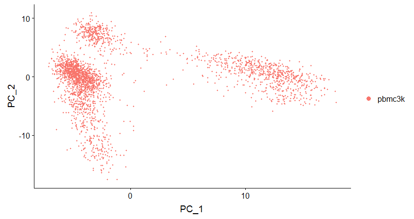
DimPlot(pbmc, reduction = "pca")

#DimHeatmap(pbmc, dims = 1, cells = 500, balanced = TRUE)
DimHeatmap(pbmc, dims = 1:15, cells = 500, balanced = TRUE)

选择多少个维度进行下一阶段的分析呢？基于PAC有以下几种方法可以探索。

# Determine the ‘dimensionality’ of the dataset 

# NOTE: This process can take a long time for big datasets, comment out for expediency. More
# approximate techniques such as those implemented in ElbowPlot() can be used to reduce
# computation time
pbmc <- JackStraw(pbmc, num.replicate = 100)
pbmc <- ScoreJackStraw(pbmc, dims = 1:20)
plot1<-JackStrawPlot(pbmc, dims = 1:15)
plot2<-ElbowPlot(pbmc)
CombinePlots(plots = list(plot1, plot2),legend="bottom")

可以看出大概在PC为十的时候，每个轴是有区分意义的。

每个轴显著相关的基因，这个也可以作为后面分析选择基因的一个参考。

#Returns a set of genes, based on the JackStraw analysis, that have statistically significant associations with a set of PCs.
?PCASigGenes
head(PCASigGenes(pbmc,pcs.use=2,pval.cut = 0.7))
[1] "PPBP"   "LYZ"    "S100A9" "IGLL5"  "GNLY"   "FTL"   

好了，最重要的一步来了，聚类分析。Seurat采用的是graph-based聚类方法，k-means方法在V3中已经不存在了。

聚类

# Cluster the cells 
#Identify clusters of cells by a shared nearest neighbor (SNN) modularity optimization based clustering algorithm. First calculate k-nearest neighbors and construct the SNN graph. Then optimize the modularity function to determine clusters. For a full description of the algorithms, see Waltman and van Eck (2013) The European Physical Journal B. Thanks to Nigel Delaney (evolvedmicrobe@github) for the rewrite of the Java modularity optimizer code in Rcpp!
pbmc <- FindNeighbors(pbmc, dims = 1:10)
pbmc <- FindClusters(pbmc, resolution = 0.5)
Modularity Optimizer version 1.3.0 by Ludo Waltman and Nees Jan van Eck

Number of nodes: 2638
Number of edges: 96033

Running Louvain algorithm...
0%   10   20   30   40   50   60   70   80   90   100%
[----|----|----|----|----|----|----|----|----|----|
**************************************************|
Maximum modularity in 10 random starts: 0.8720
Number of communities: 9
Elapsed time: 0 seconds

> table([email protected]) # 查看每一类有多少个细胞

  0   1   2   3   4   5   6   7   8 
697 483 480 344 271 162 155  32  14 
 # 提取某一类细胞。
> head(subset(as.data.frame([email protected]),[email protected]=="2"))

               [email protected]
AAACCGTGCTTCCG                 2
AAAGAGACGCGAGA                 2
AAAGCAGATATCGG                 2
AAAGTTTGTAGCGT                 2
AAATGTTGAACGAA                 2
AAATGTTGTGGCAT                 2

提取某一cluster细胞。

> pbmc
An object of class Seurat 
13714 features across 2638 samples within 1 assay 
Active assay: RNA (13714 features)
 1 dimensional reduction calculated: pca
> subpbmc<-subset(x = pbmc,idents="2")
> subpbmc
An object of class Seurat 
13714 features across 480 samples within 1 assay 
Active assay: RNA (13714 features)
 1 dimensional reduction calculated: pca

?WhichCells
head(WhichCells(pbmc,idents="2"))

[1] "AAACCGTGCTTCCG" "AAAGAGACGCGAGA" "AAAGCAGATATCGG" "AAAGTTTGTAGCGT" "AAATGTTGAACGAA" "AAATGTTGTGGCAT"
# Look at cluster IDs of the first 5 cells
head(Idents(pbmc), 5)

AAACATACAACCAC AAACATTGAGCTAC AAACATTGATCAGC AAACCGTGCTTCCG AAACCGTGTATGCG 
             1              3              1              2              6 
Levels: 0 1 2 3 4 5 6 7 8

#提取部分细胞
> pbmc
An object of class Seurat 
32738 features across 2700 samples within 1 assay 
Active assay: RNA (32738 features)
> head(colnames(pbmc@assays$RNA@counts)[1:30])
[1] "AAACATACAACCAC" "AAACATTGAGCTAC" "AAACATTGATCAGC" "AAACCGTGCTTCCG" "AAACCGTGTATGCG" "AAACGCACTGGTAC"
> subbset<-subset(x=pbmc,cells=colnames(pbmc@assays$RNA@counts)[1:30])
> subbset
An object of class Seurat 
32738 features across 30 samples within 1 assay 
Active assay: RNA (32738 features)

当然，我们用的基本都是默认参数，建议？FindClusters一下，看看具体的参数设置，比如虽然是图聚类，但是却有不同的算法，这个要看相应的文献了。

Algorithm for modularity optimization (1 = original Louvain algorithm; 2 = Louvain algorithm with multilevel refinement; 3 = SLM algorithm; 4 = Leiden algorithm). Leiden requires the leidenalg python.

系统发育分析（Phylogenetic Analysis of Identity Classes）

#Constructs a phylogenetic tree relating the 'average' cell from each identity class. 
# Tree is estimated based on a distance matrix constructed in either gene expression space or PCA spac

?BuildClusterTree
pbmc<-BuildClusterTree(pbmc)
Tool(object = pbmc, slot = 'BuildClusterTree')


Phylogenetic tree with 9 tips and 8 internal nodes.

Tip labels:
    0, 1, 2, 3, 4, 5, ...

Rooted; includes branch lengths.

PlotClusterTree(pbmc)

识别低质量样本。

#Calculate the Barcode Distribution Inflection
?CalculateBarcodeInflections
pbmc<-CalculateBarcodeInflections(pbmc)
SubsetByBarcodeInflections(pbmc)

可视化降维

非线性降维——这个目的是为了可视化，而不是特征提取（PCA），虽然它也可以用来做特征提取。

• UMAP

#Run non-linear dimensional reduction (UMAP/tSNE)
# If you haven't installed UMAP, you can do so via reticulate::py_install(packages =
# 'umap-learn')
pbmc <- RunUMAP(pbmc, dims = 1:10)

UMAP(a=None, angular_rp_forest=False, b=None, init='spectral',
   learning_rate=1.0, local_connectivity=1, metric='correlation',
   metric_kwds=None, min_dist=0.3, n_components=2, n_epochs=None,
   n_neighbors=30, negative_sample_rate=5, random_state=None,
   repulsion_strength=1.0, set_op_mix_ratio=1.0, spread=1.0,
   target_metric='categorical', target_metric_kwds=None,
   target_n_neighbors=-1, target_weight=0.5, transform_queue_size=4.0,
   transform_seed=42, verbose=True)
Construct fuzzy simplicial set
Construct embedding
    completed  0  /  500 epochs
    completed  50  /  500 epochs
    completed  100  /  500 epochs
    completed  150  /  500 epochs
    completed  200  /  500 epochs
    completed  250  /  500 epochs
    completed  300  /  500 epochs
    completed  350  /  500 epochs
    completed  400  /  500 epochs
    completed  450  /  500 epochs
> head(pbmc@[email protected]) # 提取UMAP坐标值。
                    UMAP_1    UMAP_2
AAACATACAACCAC   1.7449461 -2.770269
AAACATTGAGCTAC   4.6293025 12.092374
AAACATTGATCAGC   5.2499804 -2.011440
AAACCGTGCTTCCG -11.9875174 -1.568554
AAACCGTGTATGCG   0.1626114 -8.743275
AAACGCACTGGTAC   2.9192858 -1.487868

• t-SNE

 pbmc <- RunTSNE(pbmc, dims = 1:10)
 head(pbmc@[email protected])
                   tSNE_1     tSNE_2
AAACATACAACCAC -11.701490   7.120466
AAACATTGAGCTAC -21.981401 -21.330793
AAACATTGATCAGC  -1.292978  23.822324
AAACCGTGCTTCCG  30.877776  -9.926240
AAACCGTGTATGCG -34.619197   8.773753
AAACGCACTGGTAC  -3.046157  13.013471

比较一下两个可视化的结果。

# note that you can set `label = TRUE` or use the LabelClusters function to help label
# individual clusters
plot1<-DimPlot(pbmc, reduction = "umap",label = TRUE)+scale_color_npg()
plot2<-DimPlot(pbmc, reduction = "tsne",label = TRUE)+scale_color_npg()
CombinePlots(plots = list(plot1, plot2),legend="bottom")

可以看出，两者的降维可视化的结构是一致的，UMAP方法更加紧凑——在降维图上，同一cluster离得更近，不同cluster离得更远，作为一种后来的算法有一定的优点，但是t-SNE结构也能很好地反映cluster的空间结构。

差异分析

# Finding differentially expressed features (cluster biomarkers) 
# find all markers of cluster 1
cluster1.markers <- FindMarkers(pbmc, ident.1 = 1, min.pct = 0.25)
head(cluster1.markers, n = 5)

            p_val avg_logFC pct.1 pct.2    p_val_adj
IL32 1.894810e-92 0.8373872 0.948 0.464 2.598542e-88
LTB  7.953303e-89 0.8921170 0.981 0.642 1.090716e-84
CD3D 1.655937e-70 0.6436286 0.919 0.431 2.270951e-66
IL7R 3.688893e-68 0.8147082 0.747 0.325 5.058947e-64
LDHB 2.292819e-67 0.6253110 0.950 0.613 3.144372e-63

这是一种one-others的差异分析方法，就是cluster1与其余的cluster来做比较，当然这个是可以指定的,参数就是ident.2。

# find all markers distinguishing cluster 5 from clusters 0 and 3
cluster5.markers <- FindMarkers(pbmc, ident.1 = 5, ident.2 = c(0, 3), min.pct = 0.25)
head(cluster5.markers, n = 5)
                     p_val avg_logFC pct.1 pct.2     p_val_adj
FCGR3A        7.583625e-209  2.963144 0.975 0.037 1.040018e-204
IFITM3        2.500844e-199  2.698187 0.975 0.046 3.429657e-195
CFD           1.763722e-195  2.362381 0.938 0.037 2.418768e-191
CD68          4.612171e-192  2.087366 0.926 0.036 6.325132e-188
RP11-290F20.3 1.846215e-188  1.886288 0.840 0.016 2.531900e-184

看看输出结果都是什么。

?FindMarkers 
data.frame with a ranked list of putative markers as rows, 
and associated statistics as columns (p-values, ROC score, etc., depending on the test used (test.use)). 
The following columns are always present:

avg_logFC: log fold-chage of the average expression between the two groups. Positive values indicate that the gene is more highly expressed in the first group
pct.1: The percentage of cells where the gene is detected in the first group
pct.2: The percentage of cells where the gene is detected in the second group
p_val_adj: Adjusted p-value, based on bonferroni correction using all genes in the dataset

我们还可以输出一个总表。

# find markers for every cluster compared to all remaining cells, report only the positive ones
> pbmc.markers <- FindAllMarkers(pbmc, only.pos = TRUE, min.pct = 0.25, logfc.threshold = 0.25)
Calculating cluster 0
   |++++++++++++++++++++++++++++++++++++++++++++++++++| 100% elapsed = 08s
Calculating cluster 1
   |++++++++++++++++++++++++++++++++++++++++++++++++++| 100% elapsed = 06s
Calculating cluster 2
   |++++++++++++++++++++++++++++++++++++++++++++++++++| 100% elapsed = 21s
Calculating cluster 3
   |++++++++++++++++++++++++++++++++++++++++++++++++++| 100% elapsed = 07s
Calculating cluster 4
   |++++++++++++++++++++++++++++++++++++++++++++++++++| 100% elapsed = 08s
Calculating cluster 5
   |++++++++++++++++++++++++++++++++++++++++++++++++++| 100% elapsed = 27s
Calculating cluster 6
   |++++++++++++++++++++++++++++++++++++++++++++++++++| 100% elapsed = 21s
Calculating cluster 7
   |++++++++++++++++++++++++++++++++++++++++++++++++++| 100% elapsed = 24s
Calculating cluster 8
   |++++++++++++++++++++++++++++++++++++++++++++++++++| 100% elapsed = 19s

> head(pbmc.markers)
              p_val avg_logFC pct.1 pct.2     p_val_adj cluster  gene
RPS12 2.008629e-140 0.5029988 1.000 0.991 2.754633e-136       0 RPS12
RPS27 2.624075e-140 0.5020359 0.999 0.992 3.598656e-136       0 RPS27
RPS6  1.280169e-138 0.4673635 1.000 0.995 1.755623e-134       0  RPS6
RPL32 4.358823e-135 0.4242773 0.999 0.995 5.977689e-131       0 RPL32
RPS14 3.618793e-128 0.4283480 1.000 0.994 4.962812e-124       0 RPS14
RPS25 5.612007e-124 0.5203411 0.997 0.975 7.696306e-120       0 RPS25

> pbmc.markers %>% group_by(cluster) %>% top_n(n = 2, wt = avg_logFC)
# A tibble: 18 x 7
# Groups:   cluster [9]
       p_val avg_logFC pct.1 pct.2 p_val_adj cluster gene    
                          
 1 1.96e-107     0.730 0.901 0.594 2.69e-103 0       LDHB    
 2 1.61e- 82     0.922 0.436 0.11  2.20e- 78 0       CCR7    
 3 7.95e- 89     0.892 0.981 0.642 1.09e- 84 1       LTB     
 4 1.85e- 60     0.859 0.422 0.11  2.54e- 56 1       AQP3    
 5 0.            3.86  0.996 0.215 0.        2       S100A9  
 6 0.            3.80  0.975 0.121 0.        2       S100A8  
 7 0.            2.99  0.936 0.041 0.        3       CD79A   
 8 9.48e-271     2.49  0.622 0.022 1.30e-266 3       TCL1A   
 9 2.96e-189     2.12  0.985 0.24  4.06e-185 4       CCL5    
10 2.57e-158     2.05  0.587 0.059 3.52e-154 4       GZMK    
11 3.51e-184     2.30  0.975 0.134 4.82e-180 5       FCGR3A  
12 2.03e-125     2.14  1     0.315 2.78e-121 5       LST1    
13 7.95e-269     3.35  0.961 0.068 1.09e-264 6       GZMB    
14 3.13e-191     3.69  0.961 0.131 4.30e-187 6       GNLY    
15 1.48e-220     2.68  0.812 0.011 2.03e-216 7       FCER1A  
16 1.67e- 21     1.99  1     0.513 2.28e- 17 7       HLA-DPB1
17 7.73e-200     5.02  1     0.01  1.06e-195 8       PF4     
18 3.68e-110     5.94  1     0.024 5.05e-106 8       PPBP    

这里可以注意一下only.pos 参数，可以指定返回positive markers 基因。test.use可以指定检验方法，可选择的有：wilcox，bimod，roc，t，negbinom，poisson，LR，MAST，DESeq2。

cluster间保守conserved marker基因.

#Finds markers that are conserved between the groups
 head(FindConservedMarkers(pbmc, ident.1 = 0, ident.2 = 1, grouping.var = "groups"))
Testing group g2: (0) vs (1)
   |++++++++++++++++++++++++++++++++++++++++++++++++++| 100% elapsed = 04s
Testing group g1: (0) vs (1)
   |++++++++++++++++++++++++++++++++++++++++++++++++++| 100% elapsed = 05s
            g2_p_val g2_avg_logFC g2_pct.1 g2_pct.2 g2_p_val_adj     g1_p_val g1_avg_logFC g1_pct.1 g1_pct.2
S100A4  6.687228e-33   -0.8410733    0.678    0.959 9.170864e-29 2.583278e-35   -0.9569347    0.687    0.945
MALAT1  2.380860e-16    0.2957331    1.000    1.000 3.265112e-12 7.501490e-20    0.3201783    1.000    1.000
VIM     1.192054e-14   -0.4921326    0.816    0.951 1.634783e-10 1.193930e-19   -0.4945881    0.798    0.945
ANXA2   3.115304e-13   -0.6406856    0.169    0.461 4.272327e-09 2.186333e-18   -0.7695240    0.164    0.504
ANXA1   5.226901e-18   -0.7544607    0.451    0.800 7.168173e-14 1.413468e-17   -0.6660324    0.507    0.803
S100A11 1.832303e-16   -0.6955104    0.288    0.665 2.512820e-12 1.208765e-17   -0.7757913    0.256    0.584
        g1_p_val_adj     max_pval minimump_p_val
S100A4  3.542707e-31 6.687228e-33   5.166555e-35
MALAT1  1.028754e-15 2.380860e-16   1.500298e-19
VIM     1.637356e-15 1.192054e-14   2.387860e-19
ANXA2   2.998337e-14 3.115304e-13   4.372665e-18
ANXA1   1.938430e-13 1.413468e-17   1.045380e-17
S100A11 1.657700e-13 1.832303e-16   2.417530e-17

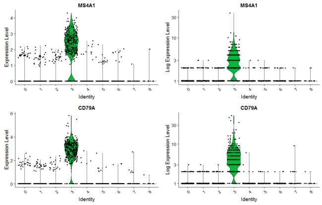
绘制基因小提琴图，其中右边的图使用原始的count取log绘制的，其实趋势还是蛮一致的。

plot1<-VlnPlot(pbmc, features = c("MS4A1", "CD79A"))+scale_color_npg()
# you can plot raw counts as well
plot2<- VlnPlot(pbmc, features = c("MS4A1", "CD79A"),ncol=1, same.y.lims=T,slot = "counts", log = TRUE)+scale_color_npg()
CombinePlots(plots = list(plot1, plot2))

plot1<-FeaturePlot(pbmc, features = c("MS4A1", "GNLY", "CD3E", "CD14", "FCER1A", "FCGR3A", "LYZ", "PPBP", 
                               "CD8A"),min.cutoff = 0, max.cutoff = 4)
top10 <- pbmc.markers %>% group_by(cluster) %>% top_n(n = 10, wt = avg_logFC)
plot2<-DoHeatmap(pbmc, features = top10$gene) + NoLegend()+scale_color_npg()
#CombinePlots(plots = list(plot1, plot2))

library(gridExtra) 
grid.arrange(plot1,plot2,ncol = 2, nrow = 1)

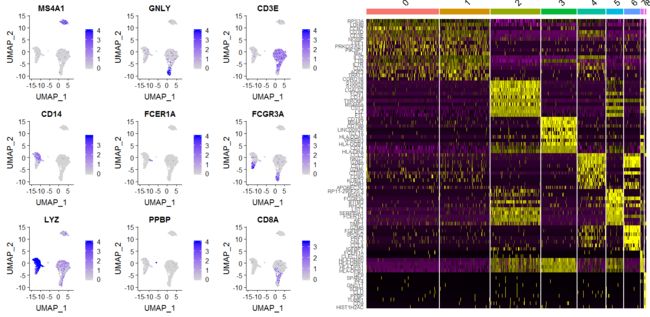
gridExtra 也是可以用来组合seurat绘制的图片的，不足为奇，seurat本身用的ggplot2语法。

细胞周期分析

与细胞周期相关的基因。

> cc.genes
$`s.genes`
 [1] "MCM5"     "PCNA"     "TYMS"     "FEN1"     "MCM2"     "MCM4"     "RRM1"     "UNG"      "GINS2"    "MCM6"    
[11] "CDCA7"    "DTL"      "PRIM1"    "UHRF1"    "MLF1IP"   "HELLS"    "RFC2"     "RPA2"     "NASP"     "RAD51AP1"
[21] "GMNN"     "WDR76"    "SLBP"     "CCNE2"    "UBR7"     "POLD3"    "MSH2"     "ATAD2"    "RAD51"    "RRM2"    
[31] "CDC45"    "CDC6"     "EXO1"     "TIPIN"    "DSCC1"    "BLM"      "CASP8AP2" "USP1"     "CLSPN"    "POLA1"   
[41] "CHAF1B"   "BRIP1"    "E2F8"    

$g2m.genes
 [1] "HMGB2"   "CDK1"    "NUSAP1"  "UBE2C"   "BIRC5"   "TPX2"    "TOP2A"   "NDC80"   "CKS2"    "NUF2"    "CKS1B"  
[12] "MKI67"   "TMPO"    "CENPF"   "TACC3"   "FAM64A"  "SMC4"    "CCNB2"   "CKAP2L"  "CKAP2"   "AURKB"   "BUB1"   
[23] "KIF11"   "ANP32E"  "TUBB4B"  "GTSE1"   "KIF20B"  "HJURP"   "CDCA3"   "HN1"     "CDC20"   "TTK"     "CDC25C" 
[34] "KIF2C"   "RANGAP1" "NCAPD2"  "DLGAP5"  "CDCA2"   "CDCA8"   "ECT2"    "KIF23"   "HMMR"    "AURKA"   "PSRC1"  
[45] "ANLN"    "LBR"     "CKAP5"   "CENPE"   "CTCF"    "NEK2"    "G2E3"    "GAS2L3"  "CBX5"    "CENPA"  

?CellCycleScoring
## Not run: 
# pbmc_small doesn't have any cell-cycle genes
# To run CellCycleScoring, please use a dataset with cell-cycle genes
# An example is available at http://satijalab.org/seurat/cell_cycle_vignette.html
pbmc <- CellCycleScoring(
  object = pbmc,
  g2m.features = cc.genes$g2m.genes,
  s.features = cc.genes$s.genes
)
head(x = [email protected])[,c(7,8,9,10,11)] # 我是为了好看取了几列来看，你大可不必。

               seurat_clusters groups     S.Score   G2M.Score Phase
AAACATACAACCAC               1     g1  0.10502807 -0.04507596     S
AAACATTGAGCTAC               3     g1 -0.02680010 -0.04986215    G1
AAACATTGATCAGC               1     g2 -0.01387173  0.07792135   G2M
AAACCGTGCTTCCG               2     g2  0.04595348  0.01140204     S
AAACCGTGTATGCG               6     g1 -0.02602771  0.04413069   G2M
AAACGCACTGGTAC               1     g2 -0.03692587 -0.08341568    G1

VlnPlot(pbmc, features = c("nFeature_RNA", "nCount_RNA", "percent.mt","percent.HB","G2M.Score","S.Score"), ncol = 6)#+scale_color_npg() 

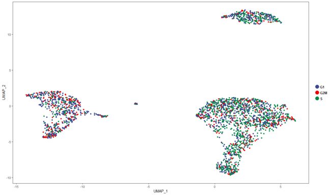
在UMAP空间中绘制细胞周期信息。

umapem<-pbmc@[email protected]
umapem<-as.data.frame(umapem)
metada= [email protected]
dim(umapem);dim(metada)

metada$bar<-rownames(metada)
umapem$bar<-rownames(umapem)
ccdata<-merge(umapem,metada,by="bar")
head(ccdata)
library(ggplot2)
plot<-ggplot(ccdata, aes(UMAP_1, UMAP_2,label=Phase))+geom_point(aes(colour = factor(Phase)))+
  #plot<-plot+scale_colour_manual(values=c("#CC33FF","Peru","#660000","#660099","#990033","black","red", "#666600", "green","#6699CC","#339900","#0000FF","#FFFF00","#808080"))+
  labs("@yunlai",x = "", y="") 
plot=plot+scale_color_aaas()  +
  theme_bw()+theme(panel.grid=element_blank(),legend.title=element_blank(),legend.text = element_text(color="black", size = 10, face = "bold"))
plot<-plot+guides(colour = guide_legend(override.aes = list(size=5))) +theme(plot.title = element_text(hjust = 0.5))

plot

探索

我们可以用SingleR或者celaref来定义每一个细胞的类型，而不只是cluster某某某了。其中SingleR与seurat是无缝衔接的，seurat对象可以读到这个里面。这里先不写，假定我们已经知道了各个类群：

# singleR 
#Assigning cell type identity to clusters
new.cluster.ids <- c("Naive CD4 T", "Memory CD4 T", "CD14+ Mono", "B", "CD8 T", "FCGR3A+ Mono", 
                     "NK", "DC", "Platelet")
names(new.cluster.ids) <- levels(pbmc)
pbmc <- RenameIdents(pbmc, new.cluster.ids)
plot1<-DimPlot(pbmc, reduction = "umap", label = TRUE, pt.size = 0.5) + NoLegend()
plot2<-DimPlot(pbmc, reduction = "tsne", label = TRUE, pt.size = 0.5) + NoLegend()
grid.arrange(plot1,plot2,ncol = 2, nrow = 1)

平均表达谱函数AverageExpression

?AverageExpression

AverageExp<-AverageExpression(pbmc,features=unique(top10$gene))
Finished averaging RNA for cluster Naive CD4 T
Finished averaging RNA for cluster Memory CD4 T
Finished averaging RNA for cluster CD14+ Mono
Finished averaging RNA for cluster B
Finished averaging RNA for cluster CD8 T
Finished averaging RNA for cluster FCGR3A+ Mono
Finished averaging RNA for cluster NK
Finished averaging RNA for cluster DC
Finished averaging RNA for cluster Platelet
> typeof(AverageExp)
[1] "list"
> head(AverageExp$RNA)
      Naive CD4 T Memory CD4 T CD14+ Mono          B      CD8 T FCGR3A+ Mono         NK         DC  Platelet
RPS3A   80.173486    61.905672 24.1161656 65.4588054 53.2413307   26.3218430 38.9542301 39.4926725 8.2843982
LDHB    13.697489    13.663320  2.5790368  2.8923463  7.1405019    1.3868494  4.4117033  3.1508971 2.0904628
CCR7     2.984692     1.293789  0.1020109  1.0788038  0.1631841    0.1413904  0.1196927  0.1473077 0.0000000
CD3D    10.724878    11.342980  0.4632153  0.3310177 13.9581981    0.2767605  1.1144081  0.2506665 0.0000000
CD3E     7.320622     7.807142  0.4356602  0.5741410  7.6701063    0.4992164  3.5389591  0.4322447 1.6960081
NOSIP    5.912196     5.196203  1.2965789  0.8373659  2.4063675    2.0503487  2.1314856  1.0916285 0.0804829

library(psych)
library(pheatmap)
coorda<-corr.test(AverageExp$RNA,AverageExp$RNA,method="spearman")
pheatmap(coorda$r)

记得保存数据以便下次使用。

saveRDS(pbmc, file = "D:\\Users\\Administrator\\Desktop\\RStudio\\single_cell\\filtered_gene_bc_matrices\\hg19pbmc_tutorial.rds")

富集分析

有了基因列表其实就可以做富集分析了借助enrichplot等R包可以做出很多好的探索。

require(org.Hs.eg.db)
library(topGO)
library(DOSE)
x=as.list(org.Hs.egALIAS2EG)
geneList<-rep(0,nrow(pbmc))
names(geneList)<-row.names(pbmc)
geneList<-geneList[intersect(names(geneList),names(x))]
newwallgenes=names(geneList)

for (ii in 1:length(geneList)){
  names(geneList)[ii]<-x[[names(geneList)[ii]]][1]
  
}


gene_erichment_results=list()
for (c1 in as.character(unique(levels(pbmc.markers$cluster)))){
  print(paste0("RUN ", c1))
  testgenes<-subset(pbmc.markers,cluster==c1)$gene
  gene_erichment_results[[c1]]=list()
  testgeneList=geneList
  testgeneList[which(newwallgenes %in% testgenes)]= 1
  #gene_erichment_results=list()
  tab1=c()
  for(ont in c("BP","MF","CC")){
    sampleGOdata<-suppressMessages(new("topGOdata",description="Simple session",ontology=ont,allGenes=as.factor(testgeneList),
                                       nodeSize=10,annot=annFUN.org,mapping="org.Hs.eg.db",ID="entrez"))
    resultTopGO.elim<-suppressMessages(runTest(sampleGOdata,algorithm="elim",statistic="Fisher"))
    
    resultTopGO.classic<-suppressMessages(runTest(sampleGOdata,algorithm="classic",statistic="Fisher"))
    tab1<-rbind(tab1,GenTable(sampleGOdata,Fisher.elim=resultTopGO.elim,Fisher.classic=resultTopGO.classic,orderBy="Fisher.elim",
                              topNodes=200))
  }
  gene_erichment_results[[c1]][["topGO"]]=tab1
  x<-suppressMessages(enrichDO(gene=names(testgeneList)[testgeneList==1],ont="DO",pvalueCutoff=1,pAdjustMethod="BH",universe=names(testgeneList),
                                minGSSize=5,maxGSSize=500,readable=T))
  gene_erichment_results[[c1]][["DO"]]=x
  dgn<-suppressMessages(enrichDGN(names(testgeneList)[testgeneList==1]))
  gene_erichment_results[[c1]][["DGN"]]=dgn
}


gene_erichment_results[["8"]][["topGO"]][1:5,]

gene_erichment_results[["1"]][["topGO"]][1:5,]
       GO.ID                                        Term Annotated Significant Expected Rank in Fisher.classic Fisher.elim Fisher.classic
1 GO:0019221         cytokine-mediated signaling pathway       516          22     4.15                      3     4.5e-05        1.4e-10
2 GO:0045059            positive thymic T cell selection        11           3     0.09                     55     7.9e-05        8.7e-05
3 GO:0050850 positive regulation of calcium-mediated ...        30           4     0.24                     61     9.1e-05        0.00010
4 GO:0033209 tumor necrosis factor-mediated signaling...        98           6     0.79                     70     0.00013        0.00016
5 GO:0002250                    adaptive immune response       301          11     2.42                     45     0.00040        3.8e-05

可视化

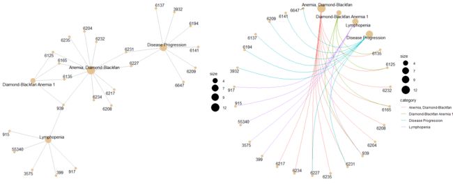
library(enrichplot)
dotplot(gene_erichment_results[[1]][["DGN"]], showCategory=30) 

## categorySize can be scaled by 'pvalue' or 'geneNum'
p1<-cnetplot(gene_erichment_results[[1]][["DGN"]], categorySize="pvalue", foldChange=geneList)
p2<-cnetplot(gene_erichment_results[[1]][["DGN"]], foldChange=geneList, circular = TRUE, colorEdge = TRUE)

plot_grid(p1, p2, ncol=2)

---

seurat v3
SeqGeq Plugins
essential_commands
R语言中S4类对象的输出方法
Salmon
Seurat - Guided Clustering Tutorial
第六章 scRNA-seq数据分析 · 生物信息学生R入门教程
computational-methods-for-single-cell-data-analysis
enrichplot