神经网络：学习（一）

代价函数（Cost Function）

在神经网络模型中，我们引入一些新的标记：

• L：表示神经网络模型的层数；
• S_l：表示第l层的激活单元的个数（注：不包括偏置单元）；
• S_L：表示输出层的激活单元的个数；
• K：表示类别分类的个数。

在正则化的逻辑回归中，其代价函数J(θ)如下：

在逻辑回归中，只有一个输出变量y，但在神经网络模型中，其输出变量是一个维度为K的向量。因此，在神经网络模型中，代价函数J(θ)改写为：

补充笔记

Cost Function

Let's first define a few variables that we will need to use:

• L = total number of layers in the network
• s_l = number of units (not counting bias unit) in layer l
• K = number of output units/classes

Recall that in neural networks, we may have many output nodes. We denote h_Θ(x)_k as being a hypothesis that results in the kth output. Our cost function for neural networks is going to be a generalization of the one we used for logistic regression. Recall that the cost function for regularized logistic regression was:

For neural networks, it is going to be slightly more complicated:

We have added a few nested summations to account for our multiple output nodes. In the first part of the equation, before the square brackets, we have an additional nested summation that loops through the number of output nodes.

In the regularization part, after the square brackets, we must account for multiple theta matrices. The number of columns in our current theta matrix is equal to the number of nodes in our current layer (including the bias unit). The number of rows in our current theta matrix is equal to the number of nodes in the next layer (excluding the bias unit). As before with logistic regression, we square every term.

Note:

• the double sum simply adds up the logistic regression costs calculated for each cell in the output layer
• the triple sum simply adds up the squares of all the individual Θs in the entire network
• the i in the triple sum does not refer to training example i

反向传播算法（Backpropagation Algorithm）

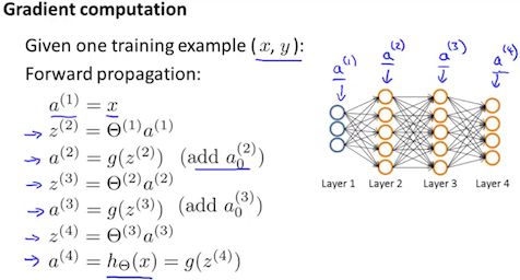
在计算h_Θ(x)时，我们采用正向传播算法，从输入层一层一层计算，直至输出层为止。

现为了计算偏导数：

我们采用反向传播算法，从输出层一层一层计算误差（误差：指激活单元的预测值a_k^(l)与实际值y_k之间的误差，其中k=1:K。），直至倒数第二层为止。最后一层为输入层，其数据时我们从训练集中获取的，所以该部分没有误差。

假设现训练集中只有一个样本，神经网络模型如下图所示：

按照反向传播算法，我们先从输出层开始计算误差，此处为了标记误差，我们引用δ来表示，则该表达式为：

这时，我们利用上述误差δ⁽⁴⁾来计算第三层的误差，其表达式为：

其中，g^'(z^(l))根据逻辑回归（二）中关于梯度下降算法的公式推导，其求导后的表达式为：

最后，我们利用δ⁽³⁾来计算第二层的误差，其表达式为：

因此，我们可以推导出代价函数J(θ)的偏导数为：

若考虑正则化以及全体样本的训练集，则我们用Δ_ij^(l)表示误差矩阵，其运算步骤如下：

将上述步骤完成后得到误差矩阵Δ_i,j^(l)：

我们便可以计算代价函数的偏导数了，其计算方法如下：

最后，我们可以得到：

由此，我们可以利用该表达式使用梯度下降算法或其他高级算法。

补充笔记

Backpropagation Algorithm

"Backpropagation" is neural-network terminology for minimizing our cost function, just like what we were doing with gradient descent in logistic and linear regression. Our goal is to compute:

That is, we want to minimize our cost function J using an optimal set of parameters in theta. In this section we'll look at the equations we use to compute the partial derivative of J(Θ):

To do so, we use the following algorithm:

Back propagation Algorithm

Given training set {(x⁽¹⁾,y⁽¹⁾)⋯(x^(m),y^(m))}

• Set Δ_i,j^(l) := 0 for all (l,i,j), (hence you end up having a matrix full of zeros)

For training example t =1 to m:

1. Set a⁽¹⁾:=x^(t)
2. Perform forward propagation to compute a^(l) for l=2,3,…,L

3. Using y(t), compute δ(L)=a(L)−y(t)

Where L is our total number of layers and a^(L) is the vector of outputs of the activation units for the last layer. So our "error values" for the last layer are simply the differences of our actual results in the last layer and the correct outputs in y. To get the delta values of the layers before the last layer, we can use an equation that steps us back from right to left:

4. Compute δ^(L−1),δ^(L−2),…,δ⁽²⁾ using δ^(l)=((Θ^(l))^Tδ^(l+1)) .∗ a^(l) .∗ (1−a^(l))

The delta values of layer l are calculated by multiplying the delta values in the next layer with the theta matrix of layer l. We then element-wise multiply that with a function called g', or g-prime, which is the derivative of the activation function g evaluated with the input values given by z^(l).

The g-prime derivative terms can also be written out as:

5. Δ_i,j^(l):=Δ_i,j^(l)+a_j^(l)δ_i^(l+1) or with vectorization, Δ^(l):=Δ^(l)+δ^(l+1)(a^(l))^T

Hence we update our new Δ matrix.

he capital-delta matrix D is used as an "accumulator" to add up our values as we go along and eventually compute our partial derivative. Thus we get:

Backpropagation Intuition

Recall that the cost function for a neural network is:

If we consider simple non-multiclass classification (k = 1) and disregard regularization, the cost is computed with:

Intuitively, δ_j^(l) is the "error" for a_j^(l) (unit j in layer l). More formally, the delta values are actually the derivative of the cost function:

Recall that our derivative is the slope of a line tangent to the cost function, so the steeper the slope the more incorrect we are. Let us consider the following neural network below and see how we could calculate some δ_j^(l):

In the image above, to calculate δ₂⁽²⁾, we multiply the weights Θ₁₂⁽²⁾ and Θ₂₂⁽²⁾ by their respective δ values found to the right of each edge. So we get δ₂⁽²⁾= Θ₁₂⁽²⁾δ₁⁽³⁾+Θ₂₂⁽²⁾δ₂⁽³⁾. To calculate every single possible δ_j^(l), we could start from the right of our diagram. We can think of our edges as our Θ_ij. Going from right to left, to calculate the value of δ_j^(l), you can just take the over all sum of each weight times the δ it is coming from. Hence, another example would be δ₂⁽³⁾=Θ₁₂⁽³⁾*δ₁⁽⁴⁾.