Risk Management
(c) Ed Seykota, 2003 & 2015
Risk
RISKis the possibility of loss. That is, if we own some stock, and there is a possibility of a price decline, we are at risk. The stock is not the risk, nor is the loss the risk. The possibility of loss is the risk.As long as we own the stock, we are at risk. The only way to control the risk is to buy or sell stock. In the matter of owning stocks, and aiming for profit, risk is fundamentally unavoidable and the best we can do is to manage the risk.
Risk Management
To manage is to direct and control. Risk management is to direct and control the possibility of loss. The activities of a risk manager are to measure risk and to increase and decrease risk by buying and selling stock.
The Coin Toss Example
Let's say we have a coin that we can toss and that it comes up heads or tails with equal probability. The Coin Toss Example helps to present the concepts of risk management .
ThePROBABILITYof an event is the likelihood of that event, expressing as the ratio of the number of actual occurrences to the number of possible occurrences. So if the coin comes up heads, 50 times out of 100, then the probability of heads is 50%. Notice that a probability has to be between zero (0.0 = 0% = impossible) and one (1.0 = 100% = certain).
Let's say the rules for the game are: (1) we start with $1,000, (2) we always bet that heads come up, (3) we can bet any amount that we have left, (4) if tails comes up, we lose our bet, (5) if heads comes up, we do not lose our bet; instead, we win twice as much as we bet, and (6) the coin is fair and so the probability of heads is 50%. This game is similar to some trading methods.
In this case, ourLUCKequals the probability of winning, or 50%; we will be lucky 50% of the time. OurPAYOFFequals 2:1 since we win 2 for every 1 we bet. OurRISKis the amount of money we wager, and therefore place at risk, on the next toss. In this example, our luck and our payoff stay constant, and only our bet may change.
In more complicated games, such as actual stock trading, luck and payoff may change with changing market conditions. Traders seem to spend considerable time and effort trying to change their luck and their payoff, generally to no avail, since it is not theirs to change. The risk is the only parameter the risk manager may effectively change to control risk.
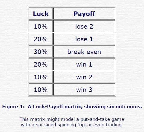
We might also model more complicated games with a matrix of lucks and payoffs, to see a range of possible outcomes. See figure 1.
For now, however, we return to our basic coin example, since it has enough dimensions to illustrate many concepts of risk management. We consider more complicated examples later.
Optimal Betting
In our coin toss example, we have constant luck at 50%, constant payoff at 2:1 and we always bet on heads. To find a risk management strategy, we have to find a way to manage the bet. This is similar to the problem confronting a risk manager in the business of trading stocks. Good managers realize that there is not much they can do about luck and payoff and that the essential problem is to determine how much to wager on the stock. We begin our game with $1,000.
Hunches and Systems
One way to determine a bet size is byHUNCH. We might have a hunch and and bet $100.
Although hunch-centric betting is certainly popular and likely accounts for an enormous proportion of actual real world betting, it has several problems: the bets require the constant attention of an operator to generate hunches, and interpret them into bets, and the bets are likely to rely as much on moods and feelings as on science.
To improve on hunch-centric betting, we might come up with a bettingSYSTEM. A system is a logical method that defines a series of bets. The advantages of a betting system, over a hunch method are (1) we don't need an operator, (2) the betting becomes regular, predictable and consistent and, very importantly, (3) we can perform a historical simulation, on a computer, toOPTIMIZEthe betting system.
Despite almost universal agreement that a system offers clear advantages over hunches, very few risk managers actually have a definition of their own risk management systems that is clear enough to allow a computer to back-test it.
Our coin-flip game, however is fairly simple and we can come up with some betting systems for it. Furthermore, we can test these systems and optimize the system parameters to find good risk management.
Fixed Bet and Fixed-Fraction Bet
Our betting system must define the bet. One way to define the bet is to make it a constant fixed amount, say $10 each time, no matter how much we win or lose. This is aFIXED BETsystem. In this case, as in fixed-betting systems in general, our $1,000EQUITYmight increase or decrease to the point where the $10 fixed bet becomes proportionately too large or small to be a good bet.
To remedy this problem of the equity drifting out of proportion to the fixed bet, we might define the bet as asFIXED-FRACTIONof our equity. A 1% fixed-fraction bet would, on our original $1,000, also lead to a $10 bet. This time, however, asour equity rises and falls, our fixed-fraction bet stays in proportion to our equity.
One interesting artifact of fixed-fraction betting, is that, since the bet stays proportional to the equity, it is theoretically impossible to go entirely broke so the official risk of total ruin is zero. In actual practice, however the disintegration of an enterprise has more to do with the psychologicalUNCLE POINT; see below.
Simulations
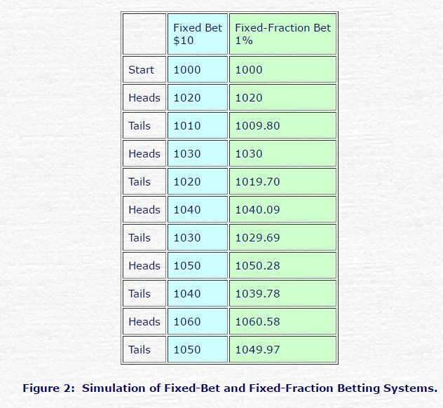
In order to test our betting system, we canSIMULATEover a historical record of outcomes. Let's say we toss the coin ten times and we come up with five heads and five tails. We can arrange the simulation in a table such as figure 2.
Notice that both systems make $20.00 (twice the bet) on the first toss, that comes up heads. On the second toss, the fixed bet system loses $10.00 while the fixed-fraction system loses 1% of $1,020.00 or $10.20, leaving $1,009.80.
Note that the results from both these systems are approximately identical. Over time, however, the fixed-fraction system grows exponentially and surpasses the fixed-bet system that grows linearly. Also note that the results depend on the numbers of heads and tails and do not at all depend on the order of heads and tails. The reader may prove this result by spreadsheet simulation.
Pyramiding and Martingale
In the case of a random process, such as coin tosses, streaks of heads or tails do occur, since it would be quite improbable to have a regular alternation of heads and tails. There is, however, no way to exploit this phenomenon, which is, itself random. In non-random processes, such as secular trends in stock prices, pyramiding and other trend-trading techniques may be effective.
Pyramiding is a method for increasing a position, as it becomes profitable. While this technique might be useful as a way for a trader to pyramid up to his optimal position, pyramiding on top of an already-optimal position is to invite the disasters of over-trading. In general, such micro-tinkering with executions is far less important than sticking to the system. To the extent that tinkering allows a window for further interpreting trading signals, it can invite hunch trading and weaken the fabric that supports sticking to the system.
The Martingale system is a method for doubling-up on losing bets. In case the doubled bet loses, the method re-doubles and so on. This method is like trying to take nickels from in front of a steam roller. Eventually, one losing streak flattens the account.
Optimizing - Using Simulation
Once we select a betting system, say the fixed-fraction betting system, we can then optimize the system by finding thePARAMETERSthat yield the bestEXPECTED VALUE. In the coin toss case, our only parameter is the fixed-fraction. Again, we can get our answers by simulation. See figures 3 and 4.
Note: The coin-toss example intends to illuminate some of the elements of risk, and their inter-relationships. It specifically applies to a coin that pays 2:1 with a 50% chance of either heads or tails, in which an equal number of heads and tails appears. It does not consider the case in which the numbers of heads and tails are unequal or in which the heads and tails bunch up to create winning and losing streaks. It does not suggest any particular risk parameters for trading the markets.
At a 0% bet there is no change in the equity. At five percent bet size, we bet 5% of $1,000.00 or $50.00 and make twice that on the first toss (heads) so we have and expected value of $1,100, shown in gray. Then our second bet is 5% of $1,100.00 or $55.00, which we lose, so we then have $1,045.00. Note that we do the best at a 25% bet size, shown in red. Note also that the winning parameter (25%) becomes evident after just one head-tail cycle. This allows us to simplify the problem of searching for the optimal parameter to the examination of just one head-tail cycle.
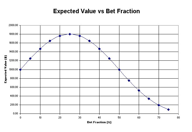
Figure 4: Expected value (ending equity) from ten tosses, versus bet fraction,for a constant bet fraction system, for a 2:1 payoff game,from the first and last columns of figure 3.
Notice that the expected value of the system rises from $1000.00 with increasing bet fraction to a maximum value of about $1,800 at a 25% bet fraction. Thereafter, with increasing bet fraction, the profitability declines. This curve expresses two fundamental principles of risk management: (1)The Timid Trader Rule: if you don't bet very much, you don't make very much, and (2)The Bold Trader Rule: If you bet too much, you go broke. In portfolios that maintain multiple positions and multiple bets, we refer to the total risk as the portfolioheat.
Note: Note the chart illustrates the Expected Value / Bet Fraction relationship for a 2:1 payoff game. For a graph of this relationship at varying payoffs, see Figure 8.
Optimizing - Using Calculus
Since our coin flip game is relatively simple, we can also find the optimal bet fraction using calculus. Since we know that the best system becomes apparent after only one head-tail cycle, we can simplify the problem to solving forjust one of the head-tail pairs.
The stake after one pair of flips:
S = (1 + b*P) * (1 - b) * S0
S - the stake after one pair of flips
b - the bet fraction
P - the payoff from winning - 2:1
S0- the stake before the pair of flips
(1 + b*P) - the effect of the winning flip
(1 - b) - the effect of the losing flip
So the effective return, R, of one pair of flips is:
R = S / S0
R = (1 + bP) * (1 - b)
R = 1 - b + bP - b2P
R = 1 + b(P-1) - b2P
Note how for small values of b, R increases with b(P-1) and how for large values of b, R decreases with b2P. These are the mathematical formulations of the timid and bold trader rules.
We can plot R versus b to get a graph that looks similar to the one we get by simulation, above, and just pick out the maximum point by inspection. We can also notice that at the maximum, the slope is zero, so we can also solve for the maximum by taking the slope and setting it equal to zero.
Slope = dR/db = (P-1) - 2bP = 0, therefore:
b = (P-1)/2P , and, for P = 2:1,
b = (2 - 1)/(2 * 2) = .25
So the optimal bet, as before, is 25% of equity.
Optimizing - Using The Kelly Formula
J. L. Kelly's seminal paper,A New Interpretation of Information Rate, 1956, examines ways to send data over telephone lines. One part of his work, The Kelly Formula, also applies to trading, to optimize bet size.
Note that the values of W and R are long-term average values,
so as time goes by, K might change a little.
Some Graphic Relationships
Between Luck, Payoff and Optimal Bet Fraction
The Optimal Bet Fraction Increases with Luck and Payoff
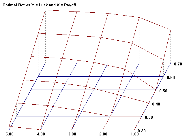
Figure 6: Optimal bet fraction increases linearly with luck, asymptotically to payoff.
This graph shows the optimal bet fraction for various values of luck (Y) and payoff (X). Optimal bet fraction increases with increasing payoff. For very high payoffs, optimal bet size equals luck. For example, for a 5:1 payoff on a 50-50 coin, the optimal bet approaches about 50% of your stake.
The Expected Value of the Process, at the Optimal Bet Fraction
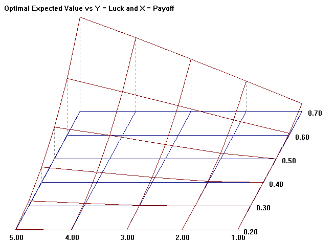
Figure 7: The optimal expected value increases with payoff and luck.
This graph shows optimal expected value for various values of luck and payoff, given betting at the optimal bet fraction. The higher the payoff (X: 1:1 to 5:1) and the higher the luck (Y: .20 to .70), the higher the expected value. For example, the highest expected value is for a 70% winning coin that pays 5:1. The lowest expected value is for a coin that pays 1:1 (even bet).
Finding the Optimal Bet Fraction from the Bet Size and Payoff
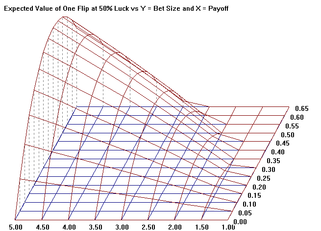
Figure 8: For high payoff, optimal bet fraction approaches luck.
This graph shows the expected value of a 50% lucky (balanced) coin for various levels of bet fraction and payoff. The expected value has an optimal bet fraction point for each level of payoff. In this case, the optimal bet fraction for a 1.5:1 payoff is about 15%; at a 2:1 payoff the optimal bet fraction is about 25%; at a 5:1 payoff, the optimal bet fraction is about 45%. Note: Figure 4 above is the cross section of figure 8, at the 2:1 payoff level.
Non-Balanced Distributions and High Payoffs
So far, we view risk management from the assumption that, over the long run, heads and tails for a 50-50 coin will even out. Occasionally, however, a winning streak does occur. If the payoff is higher than 2:1 for a balanced coin, the expected value, allowing for winning streaks, reaches a maximum for a bet-it-all strategy.
For example, for a 3:1 payoff, each toss yields an expected value of payoff-times-probability of 1.0. Therefore, the expected value for ten tosses is $1,000 x (1 + 1)10or about $1,024,000. This surpasses, by far, the expected value of about $4,200 from optimizing a 3:1 coin to about a 35% bet fraction, with the assumption of an equal distribution of heads and tails.
Almost Certain Death Strategies
Bet-it-all strategies are, by nature, almost-certain-death strategies. Since the chance of survival, for a 50-50 coin equals (.5)Nwhere N is the number of tosses, after ten tosses, the chance of survival is (.5)10, or about one chance in one thousand. Since most traders do not wish to go broke, they are unwilling to adopt such a strategy. Still, the expected value of the process is very attractive, so we would expect to find the system in use in cases where death carries no particular penalty other than loss of assets.
For example, a general, managing dispensable soldiers, might seek to optimize his overall strategy by sending them all over the hill with instructions to charge forward fully, disregarding personal safety. While the general might expect to lose many of his soldiers by this tactic, the probabilities indicate that one or two of them might be able to reach the target and so maximize the overall expected value of the mission.
Likewise, a portfolio manager might divide his equity into various sub-accounts. He might then risk 100% of each sub account, thinking that while he might lose many of them, a few would win enough so the overall expected value would maximize. This, the principle ofDIVERSIFICATION, works in cases where the individual payoffs are high.
Diversification
Diversification is a strategy to distribute investments among different securities in order to limit losses in the event of a fall in a particular security. The strategy relies on the average security having a profitable expected value, or luck-payoff product. Diversification also offers some psychological benefits to single-instrument trading since some of the short-term variation in one instrument may cancel out that from another instrument and result in an overall smoothing of short-term portfolio volatility.
The Uncle Point
From the standpoint of a diversified portfolio, the individual component instruments subsume into the overall performance. The performance of the fund, then becomes the focus of attention, for the risk manager and for the customers of the fund. The fund performance, then becomes subject to the same kinds of feelings, attitudes and management approaches that investors apply to individual stocks.
In particular, one of the most important, and perhaps under-acknowledged dimensions of fund management is theUNCLE POINTor the amount of draw down that provokes a loss of confidence in either the investors or the fundmanagement. If either the investors or the managers become demoralized and withdraw from the enterprise, then the fund dies. Since the circumstances surrounding the Uncle Point are generally disheartening, it seems to receive, unfortunately, little attention in the literature.
In particular, at the initial point of sale of the fund, the Uncle Point typically receives little mention, aside from the requisite and rather obscure notice in associated regulatory documentation. This is unfortunate, since a mismatch in the understanding of the Uncle Point between the investors and the management can lead to one or the other giving up, just when the other most needs reassurance and reinforcement of commitment.
In times of stress, investors and managers do not access obscure legal agreements, they access their primal gut feelings. This is particularly important in high-performance, high-volatility trading where draw downs are a frequent aspect of the enterprise.
Without conscious agreement on an Uncle Point, risk managers typically must assume, by default to safety, that the Uncle Point is rather close and so they seek ways to keep the volatility low. As we have seen above, safe, low volatility systems rarely provide the highest returns. Still, the pressures and tensions from the default expectations of low-volatility performance create a demand for measurements to detect and penalize volatility.
Measuring Portfolio Volatility
Sharpe, VaR, Lake Ratio and Stress Testing
From the standpoint of the diversified portfolio, the individual components merge and become part of the overall performance. Portfolio managers rely on measurement systems to determine the performance of the aggregate fund, such as the Sharpe Ratio, VaR, Lake Ratio and Stress Testing.
William Sharpe, in 1966, creates his "reward-to-variability ratio." Over time it comes to be known as the "Sharpe Ratio." The Sharpe Ratio, S, provides a way to compare instruments with different performances and different volatilities, by adjusting the performances for volatilities.
S = mean(d)/standard_deviation(d) ... the Sharpe Ratio, where
d = Rf - Rb ... the differential return, and where
Rf - return from the fund
Rb - return from a benchmark
Various variations of the Sharpe Ratio appear over time. One variation leaves out the benchmark term, or sets it to zero. Another, basically the square of the Sharpe Ratio, includes the variance of the returns, rather than the standard deviation. One of the considerations about using the Sharpe ratio is that it does not distinguish between up-side and down-side volatility, so high-leverage / high-performance systems that seek high upside-volatility do not appear favorably.
VaR, or Value-at-Risk is another currently popular way to determine portfolio risk. Typically, it measures the highest percentage draw down, that is expected to occur over a given time period, with 95% chance. The drawbacks to relying on VaR are that (1) historical computations can produce only rough approximations of forward volatility and (2) there is still a 5% chance that the percentage draw down will still exceed the expectation. Since the most severe draw down problems (loss of confidence by investors and managers) occur during these "outlier" events, VaR does not really address or even predict the very scenarios it purports to remedy.
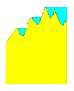
A rule-of-thumb way to view high volatility accounts, by this author, is the Lake Ratio. If we display performance as a graph over time, with peaks and valleys, we can visualize rain falling on a mountain range, filling in all the valleys. This produces a series of lakes between peaks. In case the portfolio is not at an all-time high, we also erect a dam back up to the all time high, at the far right to collect all the water from the previous high point in a final, artificial lake. The total volume of water represents the integral product of drawdown magnitude and drawdown duration.
If we divide the total volume of water by the volume of the earth below it, we have the Lake Ratio. The rate of return divided by the Lake Ratio, gives another measure of volatility-normal return. Savings accounts and other instruments that do not present draw downs do not collect lakes so their Lake-adjusted returns can be infinite.
Figure 9: The Lake Ratio = Blue / Yellow
Getting a feel for volatility by inspection.
Stress Testing
Stress Testing is a process of subjecting a model of the trading and risk management system to historical data, and noticing the historical performance, with special attention to the draw downs. The difficulty with this approach, is that few risk managers have a conscious model of their systems, so few can translate their actual trading systems to computer code. Where this is possible, however, it provides three substantial benefits (1) a framework within which to determine optimal bet-sizing strategies, (2) a high level of confidence that the systems are logical, stable and efficacious, and (3) an exhibit to support discussions to bring the risk/reward expectations of the fund managers and the investors into alignment.
The length of historical data sample for the test is likely adequate if shortening the length by a third or more has no appreciable effect on the results.
Portfolio Selection
During market cycles, individual stocks exhibit wide variations in behavior. Some rise 100 times while others fall to 1 percent of their peak values. Indicators such as the DJIA, The S&P Index, the NASDAQ and the Russell, have wide variations from each other, further indicating the importance of portfolio selection. A portfolio of the best performing stocks easily outperforms a portfolio of the worst performing stocks. In this regard, the methods for selecting the trading portfolio contribute critically to overall performance and the methodology to select instruments properly belongs in the back-testing methods.
The number of instruments in a portfolio also effects performance. A small number of instruments produces volatile, occasionally very profitable performance while a large number of instruments produces less volatile and more stable, although lower, returns.
Position Sizing
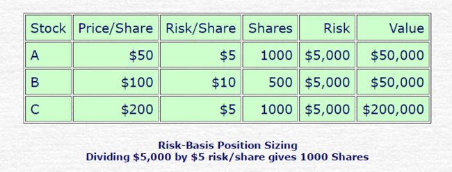
Some position sizing strategies consider value, others risk. Say a million dollar account intends to trade twenty instruments, and that the investor is willing to risk 10% of the account.
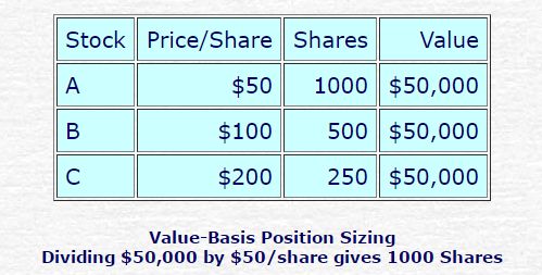
Value-Basis position sizing divides the account into twenty equal sub-accounts of $50,000 each, one for each stock. Since stocks have different prices, the number of shares for various stocks varies.
Risk-Basis position sizing considers the risk for each stock, where risk is the entry price minus the stop-out point. It divides the total risk allowance, say 10% or $100,000 into twenty sub accounts, each risking $5,000. Dividing the risk allowance, $5,000 by the risk per share, gives the number of shares.
Note that since risk per share may not be proportional to price per share (compare stocks B & C), the two methods may not indicate the same number of shares. For very close stops, and for a high risk allowance, the number of shares indicating under Risk-Basis sizing may even exceed the purchasing power of the account.
Psychological Considerations
In actual practice, the most important psychological consideration is ability to stick to the system. To achieve this, it is important (1) to fully understand the system rules, (2) to know how the system behaves and (3) to have clear and supportive agreements between all parties that support sticking to the system.
For example, as we noticed earlier, profits and losses do not likely alternate with smooth regularity; they appear, typically, as winning and losing streaks. When the entire investor-manager team realizes this as natural, it are more likely to stay the course during drawdowns, and also to stay appropriately modest during winning streaks.
In addition, seminars, support groups and other forms of attitude maintenance can help keep essential agreements on track, throughout the organization.
Risk Management - Summary
In general, good risk management combines several elements:
1. Clarifying trading and risk management systems until they can translate to computer code.
2. Inclusion of diversification and instrument selection into the back-testing process.
3. Back-testing and stress-testing to determine trading parameter sensitivity and optimal values.
4. Clear agreement of all parties on expectation of volatility and return.
5. Maintenance of supportive relationships between investors and managers.
6. Above all, stick to the system.
7. See #6, above.
