以下教程中vsearch和usearch部分的操作在虚拟机中的ubuntu18系统下进行。
1. 示例数据的下载
czh@ubuntu:~/Desktop$ curl -O https://AstrobioMike.github.io/tutorial_files/amplicon_example_workflow.tar.gz
  % Total    % Received % Xferd  Average Speed   Time    Time     Time  Current
                                 Dload  Upload   Total   Spent    Left  Speed
100 65.9M  100 65.9M    0     0   440k      0  0:02:33  0:02:33 --:--:--  497k
czh@ubuntu:~/Desktop$ tar -xzvf amplicon_example_workflow.tar.gz
czh@ubuntu:~/Desktop$ cd amplicon_example_workflow/
czh@ubuntu:~/Desktop/amplicon_example_workflow$ ls
B1_sub_R1.fq   convert_usearch_tax.sh  R1A_sub_R1.fq  R6_sub_R1.fq
B1_sub_R2.fq   primers.fa              R1A_sub_R2.fq  R6_sub_R2.fq
B2_sub_R1.fq   processing_commands.sh  R1B_sub_R1.fq  R7_sub_R1.fq
B2_sub_R2.fq   QCd_merged.fa           R1B_sub_R2.fq  R7_sub_R2.fq
B3_sub_R1.fq   R10_sub_R1.fq           R2_sub_R1.fq   R8_sub_R1.fq
B3_sub_R2.fq   R10_sub_R2.fq           R2_sub_R2.fq   R8_sub_R2.fq
B4_sub_R1.fq   R11BF_sub_R1.fq         R3_sub_R1.fq   R9_sub_R1.fq
B4_sub_R2.fq   R11BF_sub_R2.fq         R3_sub_R2.fq   R9_sub_R2.fq
BW1_sub_R1.fq  R11_sub_R1.fq           R4_sub_R1.fq   rdp_16s_v16_sp.fa
BW1_sub_R2.fq  R11_sub_R2.fq           R4_sub_R2.fq   R_working_dir
BW2_sub_R1.fq  R12_sub_R1.fq           R5_sub_R1.fq
BW2_sub_R2.fq  R12_sub_R2.fq           R5_sub_R2.fq
2. 双端reads的合并
czh@ubuntu:~/Desktop/amplicon_example_workflow$ usearch -fastq_mergepairs *_R1.fq -fastqout all_samples_merged.fq -relabel @
usearch v11.0.667_i86linux32, 4.0Gb RAM (12.0Gb total), 16 cores
(C) Copyright 2013-18 Robert C. Edgar, all rights reserved.
https://drive5.com/usearch

Merging
  Fwd B1_sub_R1.fq
  Rev B1_sub_R2.fq
  Relabel reads as B1.#

00:00 72Mb   FASTQ base 33 for file B1_sub_R1.fq
00:00 72Mb   CPU has 16 cores, defaulting to 10 threads
00:00 158Mb   100.0% 89.2% merged

Merging
  Fwd B2_sub_R1.fq
  Rev B2_sub_R2.fq
  Relabel reads as B2.#

00:00 158Mb   100.0% 88.0% merged

Merging
  Fwd B3_sub_R1.fq
  Rev B3_sub_R2.fq
  Relabel reads as B3.#

00:00 158Mb   100.0% 87.7% merged

...............................

Totals:
    212931  Pairs (212.9k)
    188162  Merged (188.2k, 88.37%)
    118298  Alignments with zero diffs (55.56%)
     24561  Too many diffs (> 5) (11.53%)
       210  Fwd tails Q <= 2 trimmed (0.10%)
         2  Rev tails Q <= 2 trimmed (0.00%)
         4  Fwd too short (< 64) after tail trimming (0.00%)
         0  Rev too short (< 64) after tail trimming (0.00%)
       204  No alignment found (0.10%)
         0  Alignment too short (< 16) (0.00%)
    211542  Staggered pairs (99.35%) merged & trimmed
    290.57  Mean alignment length
    291.22  Mean merged length
      0.31  Mean fwd expected errors
      1.37  Mean rev expected errors
      0.03  Mean merged expected errors
3. 引物剔除和数据质控
czh@ubuntu:~/Desktop/amplicon_example_workflow$ head primers.fa
>forward_primer
GTGCCAGCMGCCGCGGTAA
>reverse_primer
GGACTACHVGGGTWTCTAAT

#生成随机抽样5000条序列文件 all_sub_for_primer_check.fq
czh@ubuntu:~/Desktop/amplicon_example_workflow$ usearch -fastx_subsample all_samples_merged.fq -sample_size 5000 -fastqout all_sub_for_primer_check.fq
usearch v11.0.667_i86linux32, 4.0Gb RAM (12.0Gb total), 16 cores
(C) Copyright 2013-18 Robert C. Edgar, all rights reserved.
https://drive5.com/usearch

00:00 39Mb    100.0% Counting seqs
00:01 39Mb    100.0% Sampling

#在随机抽样文件中搜索检测引物序列
czh@ubuntu:~/Desktop/amplicon_example_workflow$ usearch -search_oligodb all_sub_for_primer_check.fq -db primers.fa -strand both -userout primer_hits.txt -userfields query+qlo+qhi+qstrand
usearch v11.0.667_i86linux32, 4.0Gb RAM (12.0Gb total), 16 cores
(C) Copyright 2013-18 Robert C. Edgar, all rights reserved.
https://drive5.com/usearch

00:00 41Mb    100.0% Reading primers.fa
00:00 7.1Mb   100.0% Masking (fastnucleo)
00:00 41Mb   CPU has 16 cores, defaulting to 10 threads
00:00 126Mb   100.0% Searching, 99.9% matched

#查看每个reads文件中检测到的引物位置
czh@ubuntu:~/Desktop/amplicon_example_workflow$ head primer_hits.txt
B1.137  1   19  +
B1.137  273 292 -
B1.486  1   19  +
B1.486  273 292 -
B1.108  1   19  +
B1.108  273 292 -
B1.429  1   19  +
B1.429  273 292 -
B1.361  1   19  +
B1.361  272 291 -
czh@ubuntu:~/Desktop/amplicon_example_workflow$ tail primer_hits.txt
R8.171761   1   19  +
R8.171761   273 292 -
R7.165730   1   19  +
R7.165730   273 292 -
R8.173376   1   19  +
R8.173376   273 292 -
R8.177799   1   19  +
R8.177799   273 292 -
R9.187451   1   19  +
R9.187451   273 292 -
#从结果中,我们可以切除reads开头的19bp和末尾的20bp从而去除引物序列。

#质控
czh@ubuntu:~/Desktop/amplicon_example_workflow$ vsearch -fastq_filter all_samples_merged.fq --fastq_stripleft 19 --fastq_stripright 20 -fastq_maxee 1 --fastq_maxlen 280 --fastq_minlen 220 --fastaout QCd_merged.fa --fastq_qmax 42
vsearch v2.10.4_linux_x86_64, 11.4GB RAM, 16 cores
https://github.com/torognes/vsearch

Reading input file 100%
186103 sequences kept (of which 186103 truncated), 2059 sequences discarded.
4. 序列去重复
czh@ubuntu:~/Desktop/amplicon_example_workflow$ vsearch --derep_fulllength QCd_merged.fa -sizeout -relabel Uniq -output unique_seqs.fa
vsearch v2.10.4_linux_x86_64, 11.4GB RAM, 16 cores
https://github.com/torognes/vsearch

Dereplicating file QCd_merged.fa 100%
46989224 nt in 186103 seqs, min 220, max 280, avg 252
Sorting 100%
93161 unique sequences, avg cluster 2.0, median 1, max 1287
Writing output file 100%
5. 聚类OTU或者产生ASVs
#剔除嵌合体并生ASVs
czh@ubuntu:~/Desktop/amplicon_example_workflow$ usearch -unoise3 unique_seqs.fa -zotus ASVs.fa -minsize 9
usearch v11.0.667_i86linux32, 4.0Gb RAM (12.0Gb total), 16 cores
(C) Copyright 2013-18 Robert C. Edgar, all rights reserved.
https://drive5.com/usearch

License: [email protected]

00:00 68Mb    100.0% Reading unique_seqs.fa
00:00 53Mb    100.0% 1549 amplicons, 3020 bad (size >= 9)
00:01 59Mb    100.0% 1542 good, 7 chimeras
00:01 59Mb    100.0% Writing zotus
6. 生成ASVs的统计表
#将文件内的每个序列的名字Zotu改为ASV开头。
czh@ubuntu:~/Desktop/amplicon_example_workflow$ sed -i.tmp 's/Zotu/ASV_/' ASVs.faczh@ubuntu:~/Desktop/amplicon_example_workflow$ head ASVs.fa
>ASV_1
TACGGAGGGGGCTAGCGTTATTCGGAATTACTGGGCGTAAAGAGTTCGTAGGCGGACTGGAAAGTTAGAGGTGAAAGCCC
AGGGCTCAACCCTGGAACGGCCTTTAAAACTTCTAGTCTAGAGACAGATAGAGGTAAGGGGAATACTTAGTGTAGAGGTG
AAATTCGTAGATATTAAGTGGAACACCAGTGGCGAAGGCGCCTTACTGGATCTGTACTGACGCTGAGGAACGAAAGCGTG
GGGAGCGAACGGG
>ASV_2
TACGAAGGTGGCGAGCGTTGTTCGGATTTACTGGGCGTAAAGAGCACGTAGGCGGTTGGGTAAGCCTCTTGGGAAAGCTC
CCGGCTTAACCGGGAAAGGTCGAGGGGAACTACTCAGCTAGAGGACGGGAGAGGAGCGCGGAATTCCCGGTGTAGCGGTG
AAATGCGTAGATATCGGGAAGAAGGCCGGTGGCGAAGGCGGCGCTCTGGAACGTACCTGACGCTGAGGTGCGAAAGCGTG
GGGAGCAAACAGG

#将每个样品的质控合并后的序列map到 ASVs.fa上。
czh@ubuntu:~/Desktop/amplicon_example_workflow$ vsearch -usearch_global QCd_merged.fa --db ASVs.fa --id 0.99 --otutabout ASV_counts.txt
vsearch v2.10.4_linux_x86_64, 11.4GB RAM, 16 cores
https://github.com/torognes/vsearch

Reading file ASVs.fa 100%
390212 nt in 1542 seqs, min 252, max 254, avg 253
Masking 100%
Counting k-mers 100%
Creating k-mer index 100%
Searching 100%
Matching query sequences: 119304 of 186103 (64.11%)
Writing OTU table (classic) 100%
7. ASVs注释
czh@ubuntu:~/Desktop/amplicon_example_workflow$ usearch -sintax ASVs.fa -db rdp_16s_v16_sp.fa -tabbedout ASV_tax_raw.txt -strand both -sintax_cutoff 0.5
usearch v11.0.667_i86linux32, 4.0Gb RAM (12.0Gb total), 16 cores
(C) Copyright 2013-18 Robert C. Edgar, all rights reserved.
https://drive5.com/usearch

License: [email protected]

00:00 62Mb    100.0% Reading rdp_16s_v16_sp.fa
00:00 28Mb    100.0% Masking (fastnucleo)
00:00 29Mb    100.0% Word stats
00:00 29Mb    100.0% Alloc rows
00:01 100Mb   100.0% Build index
00:01 133Mb  CPU has 16 cores, defaulting to 10 threads
00:01 133Mb     0.1% Processing
WARNING: s:Nitrospirillum_amazonense has parents g:Nitrospirillum (kept) and g:Azospirillum (discarded)


WARNING: s:Methanolacinia_petrolearia has parents g:Methanolacinia (kept) and g:Methanoplanus (discarded)

00:05 227Mb   100.0% Processing

#将结果文件转为为适合R语言的文件格式。
czh@ubuntu:~/Desktop/amplicon_example_workflow$ sed -i.tmp 's/#OTU ID//' ASV_counts.txt
czh@ubuntu:~/Desktop/amplicon_example_workflow$ cp ASV_counts.txt R_working_dir/
czh@ubuntu:~/Desktop/amplicon_example_workflow$ bash convert_usearch_tax.sh
czh@ubuntu:~/Desktop/amplicon_example_workflow$ cp ASV_tax.txt R_working_dir/
以下教程中R语言的操作在windows10系统下的R和Rstudio中进行。
8. R包的安装和加载
#CRAN包的安装
install.packages("vegan")
install.packages("ggplot2")
install.packages("dendextend")
install.packages("tidyr")
install.packages("viridis")
install.packages("reshape")

#Bioconductor包的安装
if (!requireNamespace("BiocManager", quietly = TRUE))
    install.packages("BiocManager")
BiocManager::install("BiocInstaller", version = "3.8")
BiocManager::install("phyloseq")
BiocManager::install("DESeq2")

#包的载入
library("phyloseq")
library("vegan")
library("DESeq2")
library("ggplot2")
library("dendextend")
library("tidyr")
library("viridis")
library("reshape")
9. 数据导入
#工作路径的设置
> getwd()
[1] "C:/Users/Administrator/Desktop/R_work"
> setwd("C:/Users/Administrator/Desktop/R_work/R_working_dir")
> list.files()
[1] "amplicon_example_analysis.R" "ASV_counts.txt"              "ASV_tax.txt"
[4] "sample_info.txt"

#数据读取
> count_tab <- read.table("ASV_counts.txt", header=T, row.names=1, check.names=F)
> tax_tab <- as.matrix(read.table("ASV_tax.txt", header=T, row.names=1, check.names=F, na.strings="", sep="\t"))
> sample_info_tab <- read.table("sample_info.txt", header=T, row.names=1, check.names=F)
> sample_info_tab
      temp    type      char
B1       blank
B2       blank
B3       blank
B4       blank
BW1    2.0   water     water
BW2    2.0   water     water
R10   13.7    rock    glassy
R11    7.3    rock    glassy
R11BF  7.3 biofilm   biofilm
R12       rock   altered
R1A    8.6    rock   altered
R1B    8.6    rock   altered
R2     8.6    rock   altered
R3    12.7    rock   altered
R4    12.7    rock   altered
R5    12.7    rock   altered
R6    12.7    rock   altered
R7        rock carbonate
R8    13.5    rock    glassy
R9    13.7    rock    glassy
10. 缺失值的处理
# first we need to get a sum for each ASV across all 4 blanks and all 16 samples
blank_ASV_counts <- rowSums(count_tab[,1:4])
sample_ASV_counts <- rowSums(count_tab[,5:20])
head(sample_ASV_counts)

# now we normalize them, here by dividing the samples' total by 4 – as there are 4x as many samples (16) as there are blanks (4)
norm_sample_ASV_counts <- sample_ASV_counts/4
head(norm_sample_ASV_counts)
# here we're getting which ASVs are deemed likely contaminants based on the threshold noted above:
blank_ASVs <- names(blank_ASV_counts[blank_ASV_counts * 10 > norm_sample_ASV_counts])
length(blank_ASVs)
# this approach identified about 50 out of ~1550 that are likely to have orginated from contamination

# looking at the percentage of reads retained for each sample after removing these presumed contaminant ASVs shows that the blanks lost almost all of their sequences, while the samples, other than one of the bottom water samples, lost less than 1% of their sequences, as would be hoped
colSums(count_tab[!rownames(count_tab) %in% blank_ASVs, ]) / colSums(count_tab) * 100

# now that we've used our extraction blanks to identify ASVs that were likely due to contamination, we're going to trim down our count table by removing those sequences and the blank samples from further analysis
filt_count_tab <- count_tab[!rownames(count_tab) %in% blank_ASVs, -c(1:4)]
# and here make a filtered sample info table that doesn't contain the blanks
filt_sample_info_tab<-sample_info_tab[-c(1:4), ]

# and let's add some colors to the sample info table that are specific to sample types and characteristics that we will use when plotting things
# we'll color the water samples blue:
filt_sample_info_tab$color[filt_sample_info_tab$char == "water"] <- "blue"
# the biofilm sample a darkgreen:
filt_sample_info_tab$color[filt_sample_info_tab$char == "biofilm"] <- "darkgreen"
# the basalts with highly altered, thick outer rinds (>1 cm) brown ("chocolate4" is the best brown I can find...):
filt_sample_info_tab$color[filt_sample_info_tab$char == "altered"] <- "chocolate4"
# the basalts with smooth, glassy, thin exteriors black:
filt_sample_info_tab$color[filt_sample_info_tab$char == "glassy"] <- "black"
# and the calcified carbonate sample an ugly yellow:
filt_sample_info_tab$color[filt_sample_info_tab$char == "carbonate"] <- "darkkhaki"

# and now looking at our filtered sample info table we can see it has an addition column for color
filt_sample_info_tab
11. β多样性
##样品数据深度标准化
# first we need to make a DESeq2 object
deseq_counts <- DESeqDataSetFromMatrix(filt_count_tab, colData = filt_sample_info_tab, design = ~type) # we have to include the colData and design arguments because they are required, as they are needed for further downstream processing by DESeq2, but for our purposes of simply transforming the data right now, they don't matter
deseq_counts_vst <- varianceStabilizingTransformation(deseq_counts)
# pulling out our transformed table
vst_trans_count_tab <- assay(deseq_counts_vst)
# and calculating our Euclidean distance matrix
euc_dist <- dist(t(vst_trans_count_tab))
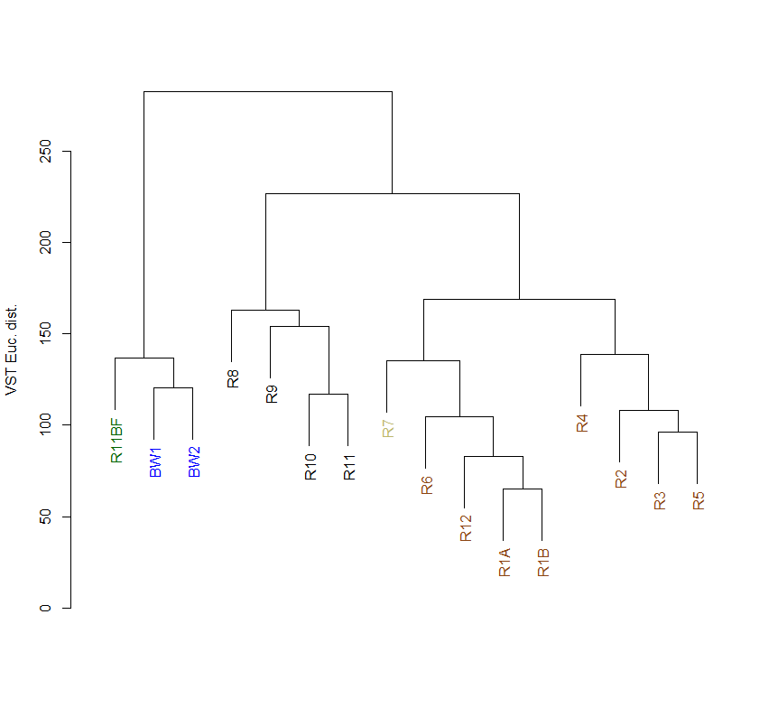
##分层聚类
euc_clust <- hclust(euc_dist, method="ward.D2")
# plot(euc_clust) # hclust objects like this can be plotted as is, but i like to change them to dendrograms for two reasons:
# 1) it's easier to color the dendrogram plot by groups
# 2) if you want you can rotate clusters with the rotate() function of the dendextend package
euc_dend <- as.dendrogram(euc_clust, hang=0.1)
dend_cols <- filt_sample_info_tab$color[order.dendrogram(euc_dend)]
labels_colors(euc_dend) <- dend_cols
plot(euc_dend, ylab="VST Euc. dist.")
PCoA分析
# making our phyloseq object with transformed table
vst_count_phy <- otu_table(vst_trans_count_tab, taxa_are_rows=T)
sample_info_tab_phy <- sample_data(filt_sample_info_tab)
vst_physeq <- phyloseq(vst_count_phy, sample_info_tab_phy)

  # generating and visualizing the PCoA with phyloseq
vst_pcoa <- ordinate(vst_physeq, method="MDS", distance="euclidean")
eigen_vals <- vst_pcoa$values$Eigenvalues # allows us to scale the axes according to their magnitude of separating apart the samples


plot_ordination(vst_physeq, vst_pcoa, color="char") +
  labs(col="type") + geom_point(size=1) +
  geom_text(aes(label=rownames(filt_sample_info_tab), hjust=0.3, vjust=-0.4)) +
  coord_fixed(sqrt(eigen_vals[2]/eigen_vals[1])) + ggtitle("PCoA") +
  scale_color_manual(values=unique(filt_sample_info_tab$color[order(filt_sample_info_tab$char)])) +
  theme(legend.position="none")
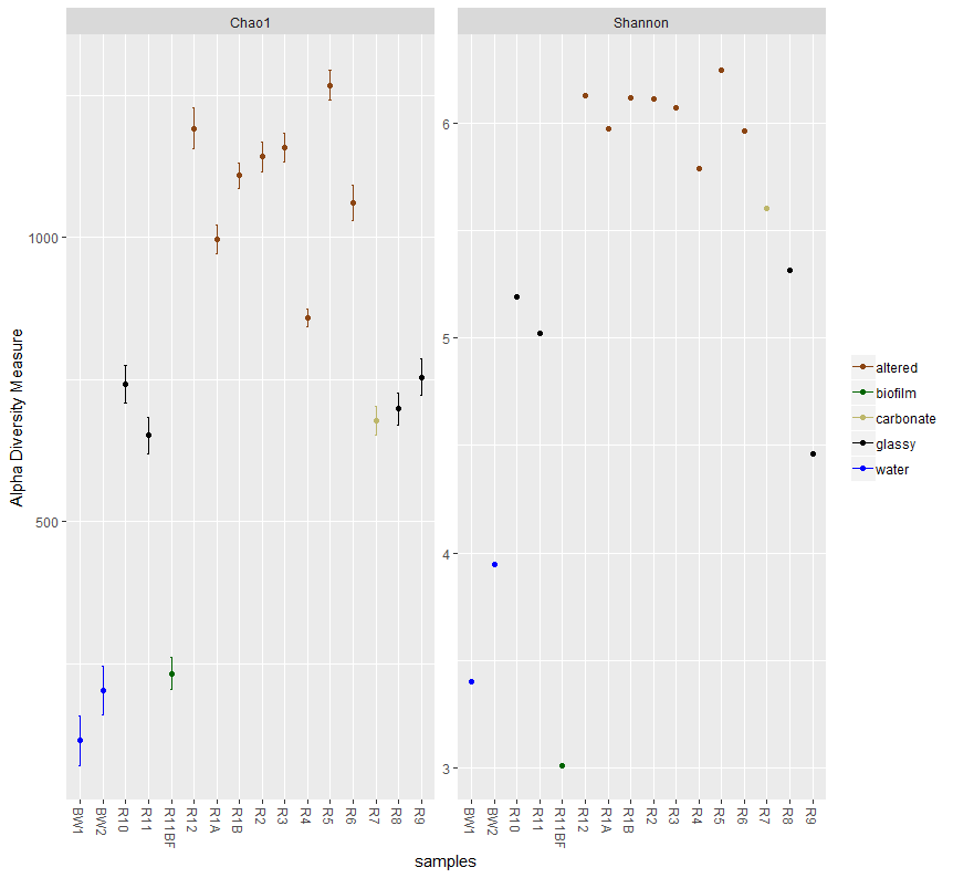
12. α多样性
#稀释曲线
rarecurve(t(filt_count_tab), step=100, col=filt_sample_info_tab$color, lwd=2, ylab="ASVs")
abline(v=(min(rowSums(t(filt_count_tab)))))
丰富度和多样性指数的计算
# first we need to create a phyloseq object using our un-transformed count table
count_tab_phy <- otu_table(filt_count_tab, taxa_are_rows=T)
tax_tab_phy <- tax_table(tax_tab)

ASV_physeq <- phyloseq(count_tab_phy, tax_tab_phy, sample_info_tab_phy)

  # and now we can call the plot_richness() function on our phyloseq object
plot_richness(ASV_physeq, color="char", measures=c("Chao1", "Shannon")) +
  scale_color_manual(values=unique(filt_sample_info_tab$color[order(filt_sample_info_tab$char)])) +
  theme(legend.title = element_blank())
plot_richness(ASV_physeq, x="type", color="char", measures=c("Chao1", "Shannon")) +
  scale_color_manual(values=unique(filt_sample_info_tab$color[order(filt_sample_info_tab$char)])) +
  theme(legend.title = element_blank())