[框架]pytorch

官方文檔

pytorch docs

安裝

建議下載anaconda創建一個新的環境(env)conda create -n pytorch_1 python=3.6，創建好後可以繳活環境activate pytorch_1，然後直接使用官網給的指令安裝(ex.conda install pytorch torchvision cudatoolkit=10.1 -c pytorch)，沒有支持CUDA的GPU可以選None。

如果要使用jupyter notebook可以conda install nb_conda用於notebook自動關聯conda，相較於tensorflow，基本上pytorch安裝不太會有CUDA以及cuDNN版本衝突的問題。
若jupyter找不到環境可以使用( python -m ipykernel install --user --name myenv --display-name "pytorch_1" )修改名稱。
查CUDA版本使用"nvcc --version"

也可以參考網路上其他教學:
windows10下安装GPU版pytorch简明教程

Tensor(張量)

Tensor 屬性
pytorch和tensorflow差不多，基本上數據都以Tensor建構。

Tensor類型

基本操作

Python本身是一門高級語言，使用很方便，但這也意味著很多操作很低效。
實際使用中應盡量調用內建函數(buildin-function)，這些函數底層由C/C++實現，能通過執行底層優化實現高效計算。因此在平時寫代碼時，就應養成向量化的思維習慣，千萬避免對較大的tensor進行逐元素遍歷。

• tensor
  tensor操作參考，基本上很多操作以及名稱都與numpy差不多，學過numpy的話應該都不是問題。
  pytorch中如果後綴＿的運算或操作為in-place(就地操作)，依照原tensor只修改有改變的相關的屬性且共用同一塊內存。
  pytorch可以與numpy相互轉換，且轉換後共用同一塊內存，修改時會一起改變，不過存在GPU(cuda:0、cuda:1...)的資料不能轉成numpy。

建立tensor

依shape建立Tensor

numpy轉換

轉換後共用內存

就地操作

clone

to()的使用

backpropagation

簡介

這邊看一個官方代碼，這是手動實現反向傳播，但既然使用tensorflow、pytorch還要手動微分求導就太麻煩了，而pytorch使用autograd來實現自動求導。

# -*- coding: utf-8 -*-

import torch

dtype = torch.float
device = torch.device("cpu")
# device = torch.device("cuda:0") # Uncomment this to run on GPU

# N is batch size; D_in is input dimension;
# H is hidden dimension; D_out is output dimension.
N, D_in, H, D_out = 64, 1000, 100, 10

# Create random input and output data
x = torch.randn(N, D_in, device=device, dtype=dtype)
y = torch.randn(N, D_out, device=device, dtype=dtype)

# Randomly initialize weights
w1 = torch.randn(D_in, H, device=device, dtype=dtype)
w2 = torch.randn(H, D_out, device=device, dtype=dtype)

learning_rate = 1e-6
for t in range(500):
    # Forward pass: compute predicted y
    h = x.mm(w1)
    h_relu = h.clamp(min=0)
    y_pred = h_relu.mm(w2)

    # Compute and print loss
    loss = (y_pred - y).pow(2).sum().item()
    print(t, loss)

    # Backprop to compute gradients of w1 and w2 with respect to loss
    grad_y_pred = 2.0 * (y_pred - y)
    grad_w2 = h_relu.t().mm(grad_y_pred)
    grad_h_relu = grad_y_pred.mm(w2.t())
    grad_h = grad_h_relu.clone()
    grad_h[h < 0] = 0
    grad_w1 = x.t().mm(grad_h)

    # Update weights using gradient descent
    w1 -= learning_rate * grad_w1
    w2 -= learning_rate * grad_w2

Computational Graphs

Calculus on Computational Graphs: Backpropagation
Tree
進入autograd 之前建議稍微先了解一下計算圖，如同tensorflow的Tensorboard所輸出的計算圖，但pytorch本身目前1.0是沒有支援計算圖可視化的(之後應該會新增)，不過pytorch是動態建立計算圖的，所以debug上沒有可視化也沒甚麼太大問題。
計算圖(Graph)由Tensor所構成的節點(node)所組成，沒有input的節點為leaf(葉子)，如果只有一個初始節點可以稱這個節點為root(根)，將他們連結的稱為邊(edge)。

Tensorboard

graph

autograd

autograd 有幾個重點:

1. 當graph存在operation node(運算節點)時就會分配buffers(緩衝區)用來存取運算的intermediary(中間結果)(如，，...)。
   然而某些運算並不需要建立buffers，ex.add、sub...。
   如果f(x) = x + w那麼df/dw是1，在這種情況下，不需要建立buffers。
   如果f(x) = x * w那麼df/dw是x，在這種情況下，我們需要建立buffers。
2. 當我們設置tensor的requires_grad=True時，表示這個node需要求導，它的所有衍生節點皆為requires_grad=True。
3. backward執行時會以執行節點進行反向傳播運算，計算後會將derivative的值傳入requires_grad=True的leaf節點，然後將buffers的intermediary清除以節省內存。
4. ""requires_grad=True的leaf node"" 以及 ""需要被用於計算intermediary(中間結果)的node""不可以使用in-place(就地操作)。
   若使用了在backward計算到這node會產生Exception，若直接取代變量不影響backward計算(backward計算是指向內存地址) 。
5. with torch.no_grad:中的所有操作視為requires_grad=False，就算requires_grad設置為True依然忽略為False。
6. detach()會傳回leaf的tensor，grad_fn會等於none，is_leaf為True，等於切斷與前面節點的連結。

補充: backward若要在運行之後保存graph及buffers，請設置retain_graph=True，設置運行完之後若要再執行記得將運算後的梯度清零避免壘加(當然若要壘加則不用)。

通常用於求完d要再次求e的時候

• 基本操作
  

  

  1
  
  
  

  2
  
  
  

  3

• 取得中間層grad
  

  

  4

• 更新權重
  

  

  5
  
  
  

  6
  
  
  

  7
  
  
  

  8

神經網絡(torch.nn)

torch.nn與tensorflow.nn以及layer類似，torch.nn裡頭封裝實現了許多神經網絡常用的運算(ex.convolution、activate function、loss function)，使我們可以更輕鬆的建立神經網絡的架構。
nn 與 nn.functional兩個是差不多的，不過一個包裝好的類，一個是可以直接調用的函數。

nn.model

使用model.parameters()取得參數(parameters)，parameters()會傳回一個generator(生成器) 。
我們可以next()、iter()、enumerate()、list()，順序會依建立model的順序排序，也可以print(model)查看。
另外named_parameters()還會附帶參數名稱，state_dict()會產生一個有序字典，可以做.keys()取得參數名稱、.values()取得參數值....等等字典的操作。

model.train（）＃把模設設成訓練模式，影響Dropout和BatchNorm
model.eval（）＃把模塊設置為預測模式，影響Dropout和BatchNorm

• 官方 範例1：

使用torch.nn.Sequential建立一個model(類似Keras)。
pytorch的conv與tensorflow默認NHWC不同，是採用nSamples x nChannels x Height x Width作為輸入尺寸。

# -*- coding: utf-8 -*-
import torch

# N is batch size; D_in is input dimension;
# H is hidden dimension; D_out is output dimension.
N, D_in, H, D_out = 64, 1000, 100, 10

# Create random Tensors to hold inputs and outputs
x = torch.randn(N, D_in)
y = torch.randn(N, D_out)

# Use the nn package to define our model as a sequence of layers. nn.Sequential
# is a Module which contains other Modules, and applies them in sequence to
# produce its output. Each Linear Module computes output from input using a
# linear function, and holds internal Tensors for its weight and bias.
model = torch.nn.Sequential(
    torch.nn.Linear(D_in, H),
    torch.nn.ReLU(),
    torch.nn.Linear(H, D_out),
)

# The nn package also contains definitions of popular loss functions; in this
# case we will use Mean Squared Error (MSE) as our loss function.
loss_fn = torch.nn.MSELoss(reduction='sum')

learning_rate = 1e-4
for t in range(500):
    # Forward pass: compute predicted y by passing x to the model. Module objects
    # override the __call__ operator so you can call them like functions. When
    # doing so you pass a Tensor of input data to the Module and it produces
    # a Tensor of output data.
    y_pred = model(x)

    # Compute and print loss. We pass Tensors containing the predicted and true
    # values of y, and the loss function returns a Tensor containing the
    # loss.
    loss = loss_fn(y_pred, y)
    print(t, loss.item())

    # Zero the gradients before running the backward pass.
    model.zero_grad()

    # Backward pass: compute gradient of the loss with respect to all the learnable
    # parameters of the model. Internally, the parameters of each Module are stored
    # in Tensors with requires_grad=True, so this call will compute gradients for
    # all learnable parameters in the model.
    loss.backward()

    # Update the weights using gradient descent. Each parameter is a Tensor, so
    # we can access its gradients like we did before.
    with torch.no_grad():
        for param in model.parameters():
            param -= learning_rate * param.grad

• 官方 範例2：

這裡我們繼承model類，必須先呼叫父類__init__，於__init__中所建構的參數(parameters)，可以被model.parameters()取得。

使用torch.nn的類建構的架構會生成一個類，並且會建立需要的參數(parameters)存於類(class)中，我們實例化後可以使用屬性取得權重或偏移值(ex. model.conv1.weight)。
torch.nn的類有定義__call__ ，我們可以給類輸入input(必須是tensor)，會return結果(也是一個tensor)，我們可以用來定義前向傳播(forward)。

---

我們也可以自行建立parameters，然後於forward中使用torch.nn.functional定義前向傳播(ex. torch.nn.functional.Conv2d)。

class Linear(nn.Module): 
    def __init__(self, in_features, out_features):
        super(Linear, self).__init__() # 呼叫父類__init__
        self.w = nn.Parameter(t.randn(in_features, out_features))
        self.b = nn.Parameter(t.randn(out_features))
    
    def forward(self, x):
        x = x.mm(self.w) # x.@(self.w)
        return x + self.b.expand_as(x)

---

建立模型：

import torch
import torch.nn as nn
import torch.nn.functional as F

class Net(nn.Module):
    def __init__(self):
        super(Net, self).__init__()
        # 1 input image channel, 6 output channels, 5x5 square convolution
        # kernel
        self.conv1 = nn.Conv2d(1, 6, 5)
        self.conv2 = nn.Conv2d(6, 16, 5)
        # an affine operation: y = Wx + b
        self.fc1 = nn.Linear(16 * 5 * 5, 120)
        self.fc2 = nn.Linear(120, 84)
        self.fc3 = nn.Linear(84, 10)

    def forward(self, x):
        # Max pooling over a (2, 2) window
        x = F.max_pool2d(F.relu(self.conv1(x)), (2, 2))
        # If the size is a square you can only specify a single number
        x = F.max_pool2d(F.relu(self.conv2(x)), 2)
        x = x.view(-1, self.num_flat_features(x))
        x = F.relu(self.fc1(x))
        x = F.relu(self.fc2(x))
        x = self.fc3(x)
        return x

    def num_flat_features(self, x):
        size = x.size()[1:]  # all dimensions except the batch dimension
        num_features = 1
        for s in size:
            num_features *= s
        return num_features

初始化(init)：

net = Net()
print(net)

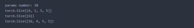
觀查模型參數：

params = list(net.parameters())
print('params number:',len(params))
print(params[0].size())  # conv1's .weight
print(params[1].size())  # conv1's .bais
print(params[2].size())  # conv2's .weight

計算前向傳播(forward)：

input = torch.randn(1, 1, 32, 32)
out = net(input)
print(out)

output = net(input)
target = torch.randn(10)  # a dummy target, for example
target = target.view(1, -1)  # make it the same shape as output
criterion = nn.MSELoss()

loss = criterion(output, target)
print(loss)

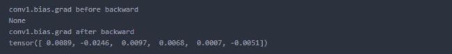
• 計算反向傳播(backward)

net.zero_grad()     # zeroes the gradient buffers of all parameters

print('conv1.bias.grad before backward')
print(net.conv1.bias.grad)

loss.backward()

print('conv1.bias.grad after backward')
print(net.conv1.bias.grad)

• 更新參數

learning_rate = 0.01
for f in net.parameters():
    f.data.sub_(f.grad.data * learning_rate)

• 範例 3 (Model 添加parameter)

import torch
import torch.nn as nn
import torch.optim as optim
class LSTM_model(nn.Module):
    def __init__(self, ):
        super(LSTM_model, self).__init__()
        self.register_parameter('w_test', nn.Parameter(nn.init.xavier_normal_(torch.zeros(300,300))))
        self.lstm0 = nn.LSTM(
            input_size=input_size,
            hidden_size=rnn_hidden_size,
            num_layers=rnn_num_layers,
            batch_first=True)
        self.linear = nn.Linear(hidden_size, hidden_size)
        self.linear0 = nn.Linear(hidden_size, output_size)
        for name,p in self.named_parameters():
            if (name.find('rnn') == 0):
                nn.init.normal_(p, mean=0.0, std=0.001)
            elif (name.find('linear') == 0) and (name.find('weight') == 0):        
                nn.init.xavier_normal_(p)
    def forward(self, x, h0,c0):
        # [b, seq, h]
        out, (h0_,c0_) = self.lstm0(x, (h0,c0))
        out = out.reshape(-1,hidden_size)
        out = self.linear(out)
        out = nn.functional.relu(out)
        out = self.linear0(out)
        out = nn.functional.softmax(out,dim=1)
        return out, (h0_,c0_)

#[rnn_layer,b,hidden_size]
batch_size=100
h0 = torch.zeros(rnn_num_layers, batch_size, rnn_hidden_size,device='cuda:0')
c0 =  torch.zeros(rnn_num_layers, batch_size, rnn_hidden_size,device='cuda:0')
model = LSTM_model()
model.cuda('cuda:0')

• 實作1
  code

優化器(torch.optim)

torch.optim
優化器與tensorflow差不多，預先設置優化器，然後使用optimizer.step()更新參數。

• 範例1：

import torch.optim as optim

# create your optimizer
optimizer = optim.SGD(net.parameters(), lr=0.01)

# in your training loop:
optimizer.zero_grad()   # zero the gradient buffers(取代前面範例的net.zero_grad())
output = net(input)
loss = criterion(output, target)
loss.backward()
optimizer.step()    # Does the update(取代前面範例的更新參數for迴圈)

• 範例2：利用字典分別設定不同parameters的學習率，這蠻方便的，比tensorflow易用許多。

  
  
  

optim.SGD([
                {'params': model.base.parameters()},
                {'params': model.classifier.parameters(), 'lr': 1e-3}
            ], lr=1e-2, momentum=0.9)

Extending PyTorch(擴展pytorch)

Extending PyTorch 官方文檔
torch.autograd.Function

• 官方 範例1：擴展一個LinearFunction

這邊解釋一下操作:

1. grad_output = dz/dy
2. dz/dx = dz/dy * dy/dx = grad_outputdy/dx = grad_outputw
3. dz/dw = dz/dy * dy/dw = grad_outputdy/dw = grad_outputx
4. dz/db = dz/dy * dy/db = grad_output*1

• saved_tensors由上下文管理器存取，saved_tensors由上下文管理器提取出來。
• ctx.needs_input_grad作為bool tuple，表示每個輸入是否需要grad。
• 如果第一個輸入到 forward() 的參數需要grad的話，ctx.needs_input_grad[0] = True。

# Inherit from Function
class LinearFunction(Function):

    # 注意: forward 與 backward 都是靜態的(@staticmethods)
    @staticmethod
    # bias is an optional(可選) argument
   #它必須接受上下文ctx作為第一個參數，後跟任意數量的參數（張量或其他類型）。
   #上下文可用於存儲張量，然後可在後向傳遞期間檢索張量。
    def forward(ctx, input, weight, bias=None):
        ctx.save_for_backward(input, weight, bias)
        output = input.mm(weight.t())
        if bias is not None:
    #unsqueeze(n維前加一個維度)，expand_as(tensor)擴展維與tensor相同形狀
            output += bias.unsqueeze(0).expand_as(output)
        return output

    # This function has only a single output, so it gets only one gradient
    @staticmethod
    #它必須接受一個上下文ctx作為第一個參數,grad_output是第2個參數
    def backward(ctx, grad_output):
        # This is a pattern that is very convenient - at the top of backward
        # unpack saved_tensors and initialize all gradients w.r.t. inputs to
        # None. Thanks to the fact that additional trailing Nones are
        # ignored, the return statement is simple even when the function has
        # optional inputs.
        input, weight, bias = ctx.saved_tensors
        grad_input = grad_weight = grad_bias = None

        # These needs_input_grad checks are optional and there only to
        # improve efficiency. If you want to make your code simpler, you can
        # skip them. Returning gradients for inputs that don't require it is
        # not an error.
        if ctx.needs_input_grad[0]:
            grad_input = grad_output.mm(weight)
        if ctx.needs_input_grad[1]:
            grad_weight = grad_output.t().mm(input)
        if bias is not None and ctx.needs_input_grad[2]:
            grad_bias = grad_output.sum(0).squeeze(0)

        return grad_input, grad_weight, grad_bias

• 官方 範例2：擴展一個Exp

class Exp(Function):
    @staticmethod
    def forward(ctx, i):
        result = i.exp()
        ctx.save_for_backward(result)
        return result
    @staticmethod
    def backward(ctx, grad_output):
        result, = ctx.saved_tensors
        return grad_output * result

• 官方教程 範例3：擴展一個ReLU

import torch


class MyReLU(torch.autograd.Function):
    """
    We can implement our own custom autograd Functions by subclassing
    torch.autograd.Function and implementing the forward and backward passes
    which operate on Tensors.
    """

    @staticmethod
    def forward(ctx, input):
        """
        In the forward pass we receive a Tensor containing the input and return
        a Tensor containing the output. ctx is a context object that can be used
        to stash information for backward computation. You can cache arbitrary
        objects for use in the backward pass using the ctx.save_for_backward method.
        """
        ctx.save_for_backward(input)
        return input.clamp(min=0)

    @staticmethod
    def backward(ctx, grad_output):
        """
        In the backward pass we receive a Tensor containing the gradient of the loss
        with respect to the output, and we need to compute the gradient of the loss
        with respect to the input.
        """
        input, = ctx.saved_tensors
        grad_input = grad_output.clone()
        grad_input[input < 0] = 0
        return grad_input


dtype = torch.float
device = torch.device("cpu")
# device = torch.device("cuda:0") # Uncomment this to run on GPU

# N is batch size; D_in is input dimension;
# H is hidden dimension; D_out is output dimension.
N, D_in, H, D_out = 64, 1000, 100, 10

# Create random Tensors to hold input and outputs.
x = torch.randn(N, D_in, device=device, dtype=dtype)
y = torch.randn(N, D_out, device=device, dtype=dtype)

# Create random Tensors for weights.
w1 = torch.randn(D_in, H, device=device, dtype=dtype, requires_grad=True)
w2 = torch.randn(H, D_out, device=device, dtype=dtype, requires_grad=True)

learning_rate = 1e-6
for t in range(500):
    # To apply our Function, we use Function.apply method. We alias this as 'relu'.
    relu = MyReLU.apply

    # Forward pass: compute predicted y using operations; we compute
    # ReLU using our custom autograd operation.
    y_pred = relu(x.mm(w1)).mm(w2)

    # Compute and print loss
    loss = (y_pred - y).pow(2).sum()
    print(t, loss.item())

    # Use autograd to compute the backward pass.
    loss.backward()

    # Update weights using gradient descent
    with torch.no_grad():
        w1 -= learning_rate * w1.grad
        w2 -= learning_rate * w2.grad

        # Manually zero the gradients after updating weights
        w1.grad.zero_()
        w2.grad.zero_()

圖形及數據轉換(torchvision.transforms)

torchvision.transforms
torchvision.transforms.functional

torchvision.transforms提供了很多圖形及數據轉換的方法，用於數據的前處理，可以使用torchvision.transforms.Compose()將它們組合在一起。

自定義Dataset

torchvision.datasets.CIFAR10
torch.utils.data.DataLoader
Training a Classifier

torch.utils.data.Dataset是一個抽象類，我們可以使用DataLoader類的__iter__方法將資料依照batch_size生成iter或enumerate，並且可以做shuffle(將數據隨機打亂)以及num_workers(使用多線程來讀數據)。

Tensor轉Dataset

我們可以使用torch.utils.data.TensorDataset(*tensor)將資料簡單的轉成Dataset ，參數可輸入多個tensor。

定義torch.utils.data.Dataset

自定義的Dataset需要繼承它並且實現兩個成員方法：

1. __getitem__()
   第一個傳入參數必須是index用來表示要取得第幾筆資料，return必須是 tensors, numbers, dicts, lists or numpy，但DataLoader都會自動處理成tensor。
2. __len__()
   return資料的長度
3. __init__()
   初始化也可不實現，但建議資料整理在init先整理好，getitem會在iter取值時才呼叫，所以會造成每次batch取值都要先call一段很長的getitem，會造成訓練時間增長，建議先在init先花時間整理好。

• 範例1
  可以參考官方CIFAR10源碼torchvision.datasets.CIFAR10如何將cifar-10-python.tar.gz整理成Dataset。

• 範例2

下面資料是之前將cifar10整理成的.npy(numpy檔案格式)。
feature資料格式是NHWC且做min max normalization[0 to 1]，labels資料格式是one-hot-encoding。
0~5共60000筆，7是經過旋轉的增量資料，noise是做autoencoder加過噪音的資料，我們將使用無噪音這些資料來定義一個Dataset。

資料

cifar-10轉npy(需要先將.gz解壓縮)：

def unpickle(file):
    import pickle
    with open(file, 'rb') as fo:
        dict = pickle.load(fo, encoding='bytes')
    return dict
def cifar_10_to_npy():
    import os
    import numpy as np
    import pandas as pd
    import pickle
    save_path = r'D:\ml_data\data_set\cifar-10-python.tar'
    cifar_dir_path = r'D:\ml_data\data_set\cifar-10-python.tar\cifar-10-batches-py'
    cifar_file_name = "data_batch_"
    cifar_path = os.path.join(cifar_dir_path,cifar_file_name)
    for num in range(1,6):
        data = unpickle(cifar_path+str(num))[b'data']
        feature = np.transpose((np.array(data)/255).astype(np.float32).reshape(-1,3,32,32),[0,2,3,1])
        np.save(os.path.join(save_path,'feature_')+str(num-1)+'.npy',feature)
        label_ = unpickle(cifar_path+str(num))[b'labels']
        label = np.array(pd.get_dummies(label_))
        np.save(os.path.join(save_path,'label_')+str(num-1)+'.npy',label)
    data = unpickle(os.path.join(cifar_dir_path,'test_batch'))[b'data']
    feature = np.transpose((np.array(data)/255).astype(np.float32).reshape(-1,3,32,32),[0,2,3,1])      
    np.save(os.path.join(save_path,'feature_5')+'.npy',feature)
    label_ = unpickle(os.path.join(cifar_dir_path,'test_batch'))[b'labels']
    label = np.array(pd.get_dummies(label_))
    np.save(os.path.join(save_path,'label_')+'.npy',label)
cifar_10_to_npy()

在windows多線程可能會有問題，建議將寫好的class存成.py然後import進來，或者設置num_workers為零不使用多線程。
DataLoader會將getitem method的return處理成tensor，這邊為了展示所以寫了一個my_transforms將x(img)轉成tensor設置好device，然後y(target)維持ndarray，建議最後next取值後在以to轉換，效能較優。

import torch
import torch.utils.data as data
import os
import numpy as np
import PIL.Image as Image
import torchvision.transforms as transforms
class Custom_Cifar10(data.Dataset):
    classes_name = ['plane', 'car', 'bird', 'cat','deer',
                    'dog', 'frog', 'horse', 'ship', 'truck']
    def __init__(self,transform=None,target_transform=None):
        self.transform = transform
        self.target_transform = target_transform
        self.data = []
        self.targets = []
        #迭代0~5筆資料依特徵及標籤分別存入data,label列表
        for num in range(6):
            X,Y = self.get_data_cifar10(num)
            self.data.append(X)
            self.targets.append(Y)
        #列表ndarray串接，NHWC to NCHW
        self.data = np.vstack(self.data)
        #列表ndarray串接
        self.targets = np.vstack(self.targets)
        
    def __getitem__(self, index):
        img, target = self.data[index], self.targets[index]
        if self.transform is not None:
            img = self.transform(img)      #x(img)轉成tensor設置好device,y(target)維持ndarray
        if self.target_transform is not None:
            target = self.target_transform(target)
        return img, target
                
    def __len__(self):
        return len(self.data)
        
    def get_data_cifar10(self,num):    #讀取數據
        """
        dir_path = D:\ml_data\data_set\cifar-10-python.tar\augment_data
        從dir_path讀取cifar資料，返回X,Y兩個numpy數組。
        共0~5組資料，參數輸入num返回第num組資料。
        """
        data_dir = r'D:\ml_data\data_set\cifar-10-python.tar\augment_data'
        data_file_name_x = 'feature_{}.npy'.format(num)
        data_file_name_y = 'label_{}.npy'.format(num)
        data_path_x = os.path.join(data_dir,data_file_name_x)
        data_path_y = os.path.join(data_dir,data_file_name_y)
        X = np.load(data_path_x)
        Y = np.load(data_path_y)
        return X,Y

def my_transforms(input):
    output = torch.tensor(input,device="cuda:0",dtype=torch.float32,requires_grad=False)
    return output

data = Custom_Cifar10(transform=my_transforms)
trainloader = torch.utils.data.DataLoader(data, batch_size=500,shuffle=True, num_workers=0)
data_iter = iter(trainloader)
x_batch = next(data_iter)[0]
y_batch = next(data_iter)[1]

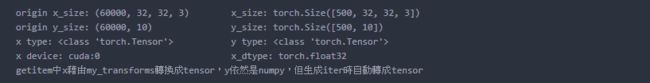
print('origin x_size:',data.data.shape,'\t x_size:',x_batch.shape)
print('origin y_size:',data.targets.shape,'\t\t y_size:',y_batch.shape)
print('x type:',type(x_batch),'\t\t y type:',type(y_batch))
print('x device:',x_batch.device,'\t\t\t x_dtype:',x_batch.dtype)
print('getitem中x藉由my_transforms轉換成tensor，y依然是numpy，但生成iter時自動轉成tensor')

數據並行

Data Parallelism
pytorch支持多GPU運行，設置也挺方便的，因為沒有多個GPU可以做範例QQ，請參考官方教程文檔。

保存與讀取model

serialization
Saving and Loading Models

• 範例1：

model、optim都有state_dict()可以傳回有序字典，可以使用load_state_dict載入。

# Define model
class TheModelClass(nn.Module):
    def __init__(self):
        super(TheModelClass, self).__init__()
        self.conv1 = nn.Conv2d(3, 6, 5)
        self.pool = nn.MaxPool2d(2, 2)
        self.conv2 = nn.Conv2d(6, 16, 5)
        self.fc1 = nn.Linear(16 * 5 * 5, 120)
        self.fc2 = nn.Linear(120, 84)
        self.fc3 = nn.Linear(84, 10)

    def forward(self, x):
        x = self.pool(F.relu(self.conv1(x)))
        x = self.pool(F.relu(self.conv2(x)))
        x = x.view(-1, 16 * 5 * 5)
        x = F.relu(self.fc1(x))
        x = F.relu(self.fc2(x))
        x = self.fc3(x)
        return x

# Initialize model
model = TheModelClass()

# Initialize optimizer
optimizer = optim.SGD(model.parameters(), lr=0.001, momentum=0.9)

# Print model's state_dict
print("Model's state_dict:")
for param_tensor in model.state_dict():
    print(param_tensor, "\t", model.state_dict()[param_tensor].size())

# Print optimizer's state_dict
print("Optimizer's state_dict:")
for var_name in optimizer.state_dict():
    print(var_name, "\t", optimizer.state_dict()[var_name])

保存

torch.save(model.state_dict(), PATH)

加載

model = TheModelClass(*args, **kwargs)
model.load_state_dict(torch.load(PATH))
model.eval()

• 範例2：直接存取變量
  

  

• 範例3：

存於GPU由CPU加載，跨設備加載可以用這類方法。

• 範例4：

保存、加載整個模型，以這種方式保存模型將使用Python的pickle模塊保存整個 模塊。