Robust PCA大法好!
Robust PCA
When dealing with high-dimensional data sets, we often leverage on the fact that the data has low intrinsic dimensionality in order to alleviate the curse of dimensionality and scale (perhaps it lies in a low-dimensional subspace or lies on a low-dimensional manifold). Principal component analysis is handy for eliminating dimensions.
Classical PCA seeks the best rank- k k estimate L L of M M (minimizing ‖M−L‖ ‖ M − L ‖ where L L has rank- k k ). Truncated SVD makes this calculation!
Traditional PCA can handle small noise, but is brittle with respect to grossly corrupted observations– even one grossly corrupt observation can significantly mess up answer.
Robust PCA factors a matrix into the sum of two matrices, M=L+S M = L + S , where M M is the original matrix, L L is low-rank, and S S is sparse. This is what we’ll be using for the background removal problem!
- Low-rank means that the matrix has a lot of redundant information– in this case, it’s the background, which is the same in every scene.
下图是原矩阵 M M (4800, 11300),4800是一帧图片60x80拉长后的向量长度,11300是帧数。图中的solid横线代表background;wave代表行人的moving;column代表 a moment in time。原矩阵 M M 每一列都是某时间点上一帧图像拉长后形成的vector,背景矩阵的rows(图中的horizontal lines)indicates L L 应当是个low-rank的矩阵;
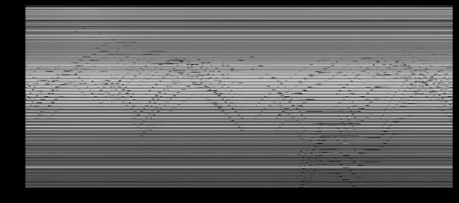
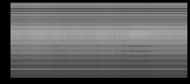
- Sparse means that the matrix has mostly zero entries– in this case, see how the picture of the foreground (the people) is mostly empty. (In the case of corrupted data, S S is capturing the corrupted entries. Assume that corrupt data is sparse).
Robust PCA的应用
Face Recognition
下图可以很明显的看到 Low-rank 矩阵就是原图,sparse 矩阵就是人工加上去的噪声!
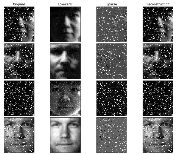
(Source: Jean Kossaifi)
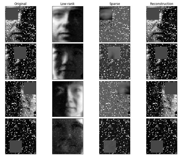
(Source: Jean Kossaifi)
Robust PCA Optimization
Source
The general primary component pursuit algorithm from this Robust PCA paper (Candes, Li, Ma, Wright), in the specific form of Matrix Completion via the Inexact ALM Method found in section 3.1 of this paper (Lin, Chen, Ma).
Optimize Algorithms
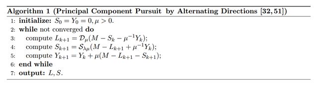
I. principal component pursuit
Robust PCA can be written:
where:
‖⋅‖1 ‖ ⋅ ‖ 1 is the L1 norm. Minimizing the L1 norm results in sparse values. For a matrix, the L1 norm is equal to the maximum absolute column norm.
- Q:这里为啥用 L1 L 1 norm呢?
因为 L1 L 1 norm会lead更好的稀疏性,而我们需要 S S to be a sparse matrix.
‖⋅‖∗ ‖ ⋅ ‖ ∗ is the nuclear norm, which is the L1 norm of the singular values. Trying to minimize this results in sparse singular values –> low rank.

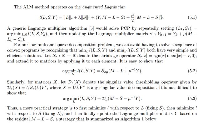
shrinkage operator Sτ[x]=sgn(x)max(|x|−τ,0) S τ [ x ] = sgn ( x ) max ( | x | − τ , 0 )
取 S S 中的singular value,然后减去 τ τ ,如果value比 τ τ 小,就round them to 0. 如果 value 大于 τ τ 就将两者的差反号,使得singular value更接近0。总的来说这个shrinkage操作就是使得singular value smaller,从而使它们更加sparse。不要忘了我们的目标是:找到一个sparse的 S S 。singular value thresholder D D
就是先对矩阵做SVD分解,然后通过 S S 的 shrinkage 操作使得singular value变小之后,再reconstruct Dτ(X)=USτ(∑)V∗ D τ ( X ) = U S τ ( ∑ ) V ∗ 得到Low_rank矩阵 L L 的approximation。这个操作有点像 truncated SVD,也就是说把singular value比较小(小于 τ τ )的那些vector cut off。
第3、4步的意思大概是,因为我们的目标是要把原矩阵分解成一个 Low_rank 矩阵 L L 加上一个 Sparse 矩阵 S S ,所以这里我们要不断让 Low_rank矩阵等于原矩阵 M M 减去 Sparse 矩阵 S S ,同时让 S S 尽可能等于 M−L M − L 。是一个比较典型的交替更新的方法。
而 μ−1Yk μ − 1 Y k 是为了 keep track of what you still have to approximate(residual error).
II. ALM
Section 3.1 of Chen, Lin, Ma contains a faster vartiation of this:
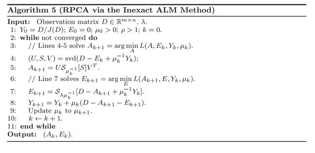
And Section 4 has some very helpful implementation details on how many singular values to calculate (as well as how to choose the parameter values):
Implement principal component pursuit
借用 Facebook’s Fast Randomized PCA library实现一发principal component pursuit。
from scipy import sparse
from sklearn.utils.extmath import randomized_svd
import fbpca

# TOL是收敛的boundary
TOL=1e-9
MAX_ITERS=3

def converged(Z, d_norm):
    err = np.linalg.norm(Z, 'fro') / d_norm
    print('error: ', err)
    return err < TOL
shrinkage operator:把小于 τ τ 的singular value都置为0,从另一角度来看就是类似在truncating matrix,ignore那些很小的singular value。
def shrink(M, tau):
    S = np.abs(M) - tau
    return np.sign(M) * np.where(S>0, S, 0)
# 写作pca, 读作svd,实际上是一个fast svd implementation
def _svd(M, rank): return fbpca.pca(M, k=min(rank, np.min(M.shape)), raw=True)
def norm_op(M): return _svd(M, 1)[1][0]
# D操作
# 这里的rank是因为fbpca.pca做的是randomized svd,所以需要指定你要保留的rank数
def svd_reconstruct(M, rank, min_sv):
u, s, v = _svd(M, rank)
# 这里面min_sv就是下面提到的sv
s -= min_sv
nnz = (s > 0).sum()
return u[:,:nnz] @ np.diag(s[:nnz]) @ v[:nnz], nnzprincipal component pursuit关键代码实现:
# principal component pursuit是Robust PCA的其中一种algorithm
def pcp(X, maxiter=10, k=10): # refactored
m, n = X.shape
trans = mif trans: X = X.T; m, n = X.shape
lamda = 1/np.sqrt(m)
op_norm = norm_op(X)
Y = np.copy(X) / max(op_norm, np.linalg.norm( X, np.inf) / lamda)
mu = k*1.25/op_norm; mu_bar = mu * 1e7; rho = k * 1.5
d_norm = np.linalg.norm(X, 'fro')
L = np.zeros_like(X); sv = 1
examples = []
for i in range(maxiter):
print("rank sv:", sv)
X2 = X + Y/mu
# update estimate of Sparse Matrix by "shrinking/truncating": original - low-rank
# 对应step 4
S = shrink(X2 - L, lamda/mu)
# update estimate of Low-rank Matrix by doing truncated SVD of rank sv & reconstructing.
# count of singular values > 1/mu is returned as svp
# 对应step 3
L, svp = svd_reconstruct(X2 - S, sv, 1/mu)
'''
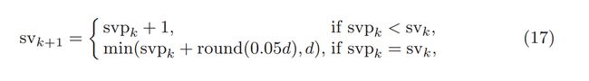
这个sv是个划重点的东西,代表了你在truncating svd希望保留的rank数目,这个值需要不停地更新
原始矩阵为400*11300,很明显我们不可能做full svd,肯定贼慢
所以我们先甩掉singular value小于1/μ对应的那些vector,
* 如果我们得到的rank:svp < sv,说明我们想要的value(不小于1/μ的)都已经保留了,
即我们甩掉的value都是该甩的,则下一轮只将 sv + 1(因为第sv之后的singular value也没包含太多信息了)
* 否则即 svp = sv 说明第sv个singular value之后的value可能还有大于1/μ的,
我们甩多了,所以下一轮就要多保留一些sv
看Results中的输出来check一下
'''
# If svp < sv, you are already calculating enough singular values.
# If not, add 20% (in this case 240) to sv
sv = svp + (1 if svp < sv else round(0.05*n))
# residual
Z = X - L - S
Y += mu*Z; mu *= rho
# keep track Time=140 时的visual
examples.extend([S[140,:], L[140,:]])
if m > mu_bar: m = mu_bar
if converged(Z, d_norm): break
if trans: L=L.T; S=S.T
return L, S, examples Results
m, n = M.shape
round(m * .05)

#240
L, S, examples = pcp(M, maxiter=5, k=10)rank sv: 1
error: 0.131637937114
rank sv: 241
error: 0.0458515689041
rank sv: 49
error: 0.00588796042886
rank sv: 289
error: 0.000565564416732
rank sv: 529
error: 2.47254909523e-05sv 初始化为 1,然后加上 n 的 20%,即 240。
然后 svp = 48 < 241,所以 sv = 48 + 1 =49。