【自然语言处理】聊聊注意力机制(Attention Mechanism)的发展
前言
其实,关于注意力机制的文章真的有很多,而且写得相当精彩(毕竟过去这么多年了),这篇博文的主要目的在于以一个不同的角度(理论+代码)阐述注意力机制。
浅谈
首先这件事还要从序列到序列模型(Seq2seq Model)开始说起,最早的序列到序列模型是一个CNN+LSTM。
简单来说就是把CNN把编码端映射成一个固定向量,然后用LSTM一步步解码。
接着一个自然的想法是使用LSTM[1],因为LSTM的处理序列能力更强嘛。那么一种简单的做法是将编码端的最后一个隐层状态作为解码端的初始状态。

那么很明显最后一个隐层的状态(固定长度的向量)随着句子长度正常携带的信息能力会明显不足。
为了解决这个问题,引入注意力机制,在解码端的每一步都得到一个创建一个 上 下 文 向 量 \color{red}{上下文向量} 上下文向量(Context Vector),通过上下文向量和解码端的输入生成下一个词。
而Transformer的自注意力机制(Self-Attention)就是将注意力机制从编码端到解码端抽取出来,使其可以捕获句子间的关系,实验证明了这种效果确实比LSTM好太多。
如果你只是单纯想了解下Attention,那么浅谈看看就够了,如果想深入,请往下继续看。(前方高能)
深入了解
Bahdanau Attention
第一个注意力机制,称为Bahdanau Attention[2]。
记编码器(Encoder)的隐含状态为 h h h,记解码器(Decoder)的隐含状态为 s s s。

p ( y i ∣ y 1 , . . . , y i − 1 , x ) = g ( y i − 1 , s i , c i ) p(y_i|y_1,...,y_{i-1},x)=g(y_{i-1},s_i,c_i) p(yi∣y1,...,yi−1,x)=g(yi−1,si,ci)
首先解码器当前词 y i y_i yi的输出根据上一个词 y i 1 y_{i_1} yi1,上一个解码器的隐含状态为 s i s_i si以及上下文向量 c i c_i ci得到。
s i = f ( s i − 1 , y i − 1 , c i ) s_i=f(s_{i-1},y_{i-1},c_i) si=f(si−1,yi−1,ci)
那么,解码器当前隐含层状态 s i s_i si则跟上一个隐含层状态 s i − 1 s_{i-1} si−1,上一个输出 y i − 1 y_{i-1} yi−1和当前的上下文向量 c i c_i ci。
c i = ∑ j = 1 T x a i j h j c_i=\sum\limits_{j=1}^{T_x} {a_{ij}h_j} ci=j=1∑Txaijhj
当前的上下文向量 c i c_i ci是加权求和,注意到 T x T_x Tx是编码器层的步长,而 a i j a_{ij} aij表示这个编码器的隐含层构成上下文向量的一个权重。
a i j = e x p ( e i j ) ∑ k = 1 T x e x p ( e i k ) a_{ij}=\frac{exp(e_{ij})}{\sum\limits_{k=1}^{T_x}exp(e_{ik})} aij=k=1∑Txexp(eik)exp(eij)
那么 a i j a_{ij} aij则是通过 e i j e_{ij} eij的softmax得到。
以及 e i j = a ( s i − 1 , h j ) e_{ij}=a(s_{i-1},h_j) eij=a(si−1,hj)
这里的 e i j e_{ij} eij可以意味着解码器的前一个隐层状态 s i − 1 s_{i-1} si−1和编码器的某一个隐层状态 h j h_j hj的一个相似度,这里是用的一个前馈网络得到。
memory是encoder_outputs,也就是编码器的所有隐层状态,query。
来瞅瞅Tensorflow的代码。 BahdanauAttention代码
    score = _bahdanau_score(
          processed_query,
          self._keys,
          attention_v,
          attention_g=attention_g,
          attention_b=attention_b)
    alignments = self._probability_fn(score, state)
    next_state = alignments
这里的score就是 a j a_j aj, a j a_j aj的大小是一个编码器层步长 T x T_x Tx的向量。
def _bahdanau_score(processed_query,
                    keys,
                    attention_v,
                    attention_g=None,
                    attention_b=None):
  """Implements Bahdanau-style (additive) scoring function.
  This attention has two forms.  The first is Bhandanau attention,
  as described in:
  Dzmitry Bahdanau, Kyunghyun Cho, Yoshua Bengio.
  "Neural Machine Translation by Jointly Learning to Align and Translate."
  ICLR 2015. https://arxiv.org/abs/1409.0473
  The second is the normalized form.  This form is inspired by the
  weight normalization article:
  Tim Salimans, Diederik P. Kingma.
  "Weight Normalization: A Simple Reparameterization to Accelerate
   Training of Deep Neural Networks."
  https://arxiv.org/abs/1602.07868
  To enable the second form, set please pass in attention_g and attention_b.
  Args:
    processed_query: Tensor, shape `[batch_size, num_units]` to compare to keys.
    keys: Processed memory, shape `[batch_size, max_time, num_units]`.
    attention_v: Tensor, shape `[num_units]`.
    attention_g: Optional scalar tensor for normalization.
    attention_b: Optional tensor with shape `[num_units]` for normalization.
  Returns:
    A `[batch_size, max_time]` tensor of unnormalized score values.
  """
  # Reshape from [batch_size, ...] to [batch_size, 1, ...] for broadcasting.
  processed_query = array_ops.expand_dims(processed_query, 1)
  if attention_g is not None and attention_b is not None:
    normed_v = attention_g * attention_v * math_ops.rsqrt(
        math_ops.reduce_sum(math_ops.square(attention_v)))
    return math_ops.reduce_sum(
        normed_v * math_ops.tanh(keys + processed_query + attention_b), [2])
  else:
    return math_ops.reduce_sum(
        attention_v * math_ops.tanh(keys + processed_query), [2])
而这个分数的计算则是通过processed_query(编码器所有隐层状态, T x T_x Tx个),keys(编码器当前的隐层状态,1个),论文提到是一个前馈网络,所以这里使用tanh激活函数。
Loung Attention
第二个注意力机制,是继Bahdanau Attention后的一个注意力机制叫Loung Attention[4]。
记编码器(Encoder)的隐含状态为 h t h_t ht,记解码器(Decoder)的隐含状态为 h s h_s hs。(请注意,跟Bahdanau Attention不一样了)

首先说说他们的区别。
第一,Loung Attention提供了两种的注意力机制,一个是全局注意力机制(Global Attention),考虑全部的编码器的隐含状态;一个是局部注意力机制(Local Attention),只考虑局部窗口的隐含状态,这样可以节省计算量。
第二,全局注意力机制和Bahdanau Attention相似,但是还是有些区别,一个是Bahdanau Attention的编码器隐含层是由一个双向LSTM然后拼接而成, h i = [ h → i ; h ← j ] h_i=[\overrightarrow h_i; \overleftarrow h_j] hi=[hi;hj],而Loung Attention仅仅是用了最顶层的隐含层。二个,两者计算解码器隐含层状态不同。Bahdanau Attention是 h t − 1 → a t → c t → h t h_{t-1} \to a_t \to c_t \to h_t ht−1→at→ct→ht,Loung Attention是 h t → a t → c t → h ~ t h_{t} \to a_t \to c_t \to \tilde h_t ht→at→ct→h~t,简单来讲,Loung Attention像Seq2seq一样先计算出解码层的隐含状态 h t h_t ht,再结合上下文向量 c t c_t ct得出最终的解码器隐含状态(后文我把它称为解码器顶层隐含状态) h ~ t \tilde h_t h~t。
p ( y t ∣ y < t , x ) = s o f t m a x ( W s h ~ t ) p(y_t|y_{
我们可以看到生成下一个词的主要是依靠这个当前的顶层解码器隐层状态 h ~ t \tilde h_t h~t。
h ~ t = t a n h ( W c [ c t ; h t ] ) \tilde h_t = tanh(W_c[c_t;h_t]) h~t=tanh(Wc[ct;ht])
而这个当前的顶层解码器隐层状态则是根据当前上下文向量 c t c_t ct和解码器隐含层状态 h t h_t ht得到。
A t ( s ) = a l i g n ( h t , h s ) = e x p ( s c o r e ( h t , h ˉ s ) ) ∑ s ’ e x p ( s c o r e ( h t , h ˉ s ) \begin{array}{c} A_t(s) = align(h_t,h_s)\\ = \frac {exp(score(h_t,\bar h_s))}{\sum\nolimits_{s^’} {exp(score(h_t,\bar h_s)}} \end{array} At(s)=align(ht,hs)=∑s’exp(score(ht,hˉs)exp(score(ht,hˉs))
其实 c t c_t ct的创建跟Bahdanau Attention类似,主要是计算 a i j a_{ij} aij的方式有些不同。并且Loung Attention提供了三种计算分数(score)的方式。
LuongAttention代码
    with variable_scope.variable_scope(None, "luong_attention", [query]):
      attention_g = None
      if self._scale:
        attention_g = variable_scope.get_variable(
            "attention_g",
            dtype=query.dtype,
            initializer=init_ops.ones_initializer,
            shape=())
      score = _luong_score(query, self._keys, attention_g)
    alignments = self._probability_fn(score, state)
    next_state = alignments
def _luong_score(query, keys, scale):
  """Implements Luong-style (multiplicative) scoring function.
  This attention has two forms.  The first is standard Luong attention,
  as described in:
  Minh-Thang Luong, Hieu Pham, Christopher D. Manning.
  "Effective Approaches to Attention-based Neural Machine Translation."
  EMNLP 2015.  https://arxiv.org/abs/1508.04025
  The second is the scaled form inspired partly by the normalized form of
  Bahdanau attention.
  To enable the second form, call this function with `scale=True`.
  Args:
    query: Tensor, shape `[batch_size, num_units]` to compare to keys.
    keys: Processed memory, shape `[batch_size, max_time, num_units]`.
    scale: the optional tensor to scale the attention score.
  Returns:
    A `[batch_size, max_time]` tensor of unnormalized score values.
  Raises:
    ValueError: If `key` and `query` depths do not match.
  """
  depth = query.get_shape()[-1]
  key_units = keys.get_shape()[-1]
  if depth != key_units:
    raise ValueError(
        "Incompatible or unknown inner dimensions between query and keys.  "
        "Query (%s) has units: %s.  Keys (%s) have units: %s.  "
        "Perhaps you need to set num_units to the keys' dimension (%s)?" %
        (query, depth, keys, key_units, key_units))

  # Reshape from [batch_size, depth] to [batch_size, 1, depth]
  # for matmul.
  query = array_ops.expand_dims(query, 1)

  # Inner product along the query units dimension.
  # matmul shapes: query is [batch_size, 1, depth] and
  #                keys is [batch_size, max_time, depth].
  # the inner product is asked to **transpose keys' inner shape** to get a
  # batched matmul on:
  #   [batch_size, 1, depth] . [batch_size, depth, max_time]
  # resulting in an output shape of:
  #   [batch_size, 1, max_time].
  # we then squeeze out the center singleton dimension.
  score = math_ops.matmul(query, keys, transpose_b=True)
  score = array_ops.squeeze(score, [1])

  if scale is not None:
    score = scale * score
  return score
主要看这句代码。
score = math_ops.matmul(query, keys, transpose_b=True)
这里的分数就是内积,也就是Attention分数计算方式之一。
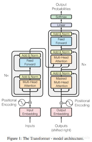
Self-Attention
自注意力机制是Transformer[4]提出的。以上在代码里面query,key,value都是这篇文章提出的一些概念,就是这篇文章把注意力机制给抽取出来,把它变得更通用、一般化了。
可以注意每一个Transformer块(Block)都有一个Add&Norm,这里面用到了残差网络(Residual Network)和批量归一化(Batch Normalization)。批量归一化就是将输入 X X X进行归一化,使得输入数据能够服从同一分布。
一般的来讲key和value代表着之前编码器端的隐含状态,query指代解码器端的隐含状态。那么注意力机制就是用key跟query计算得到一个权重矩阵(之前的score)然后跟value进行加权求出一个上下文向量。
A t t e n t i o n ( Q , K , V ) = s o f t m a x ( Q K T d k ) V Attention(Q,K,V)=softmax(\frac{QK^T}{\sqrt d_k})V Attention(Q,K,V)=softmax(dkQKT)V
主要看下Attention的计算,其实这里会发现这个跟之前的Attention计算方式非常相似, Q K T QK^T QKT的结果就类似一个score,但是这里多了一个缩放因子 d k \sqrt d_k dk,文章提到是用来缩放的,避免score太大,会把概率分化接近成1和0。
这里的Transformer的计算不过多阐述,具体可以看 图解Transformer。
总结
目前好多论文似乎都要"注意力机制"一下,不过也间接地证明了注意力机制的有效性。其实目前的一些ELMO把词向量从静态走向动态,其中使用了加权得到的词向量的思想跟注意力机制非常相似,所以了解注意力机制的本质对后面的论文的帮助还是非常大的。
参考文献
【1】Sutskever I, Vinyals O, Le Q V. Sequence to sequence learning with neural networks[C]//Advances in neural information processing systems. 2014: 3104-3112.
【2】Bahdanau D, Cho K, Bengio Y. Neural machine translation by jointly learning to align and translate[J]. arXiv preprint arXiv:1409.0473, 2014.
【3】Luong M T, Pham H, Manning C D. Effective approaches to attention-based neural machine translation[J]. arXiv preprint arXiv:1508.04025, 2015.
【4】Vaswani A, Shazeer N, Parmar N, et al. Attention is all you need[C]//Advances in neural information processing systems. 2017: 5998-6008.