Introduction to SPM statistics
目录
- Introduction to SPM statistics
- Introduction
- Naming of parts
- PET and fMRI
- An example analysis in SPM
- Step one: getting the data from the images
- Step two: getting the data ready to analyse
- Global image signal
- Grand mean scaling
- Statistics: the simplest case - a regression
- From model to matrices
- t statistics and contrasts
- A short note on hypothesis testing
- From t statistics to Z scores
- More than one covariate
- Adding conditions: the General Linear Model
- The end
This page is a basic introduction to the statistics in SPM. It refers to SPM versions 96 and later. The page is designed for readers who have had very little formal statistical background, and I have tried to keep formulae to a minimum. You will not need any knowledge of the matlab programming language to understand the page, but if you do know matlab then you will probably want to refer to the code that I have used to create the figures. The code is contained in the http://imaging.mrc-cbu.cam.ac.uk/scripts/statstalk.m script, and contains several example pieces of code for obtaining and analysing image data. There are instructions in the script on the steps you will need to follow to allow you to run it.
For a more technical treatment of the statistical background of SPM, that I found very useful, see the chapter on the general linear model in the Human Brain Function book - second edition.
You can also watch the videos of the SPM Course for fMRI, PET and VBM, at the Wellcome Trust Centre for Neuroimaging (May 2011).
Introduction
The statistics interface to SPM, it should be said, is not easy to understand for the first-time user. This fact is more surprising than it may seem, because SPM uses much of the same underlying maths as many other statistics packages, such as SPSS. The reason that the statistical interface to SPM is so much harder to understand is that SPM chooses to take the user much closer to the maths; it sacrifices ease of understanding for enormous flexiblity of the designs that can be analysed with the same interface. To understand the SPM interface, you will need some understanding of the underlying maths. I hope to show that this need not be an insurmountable task, even for the relative statistical novice.To start, it is important to point out that SPM creates statistics by doing a seperate statistical analysis for each voxel. Like most other functional imaging programs, SPM analyses each voxel independently. Specifically, it:
does an analysis of variance separately at each voxel;
- makes t statistics from the results of this analysis, for each voxel;
- works out a Z score equivalent for the t statistic;
- shows you an image of the t statistics (SPM99), or equivalent Z scores (SPM96);
- suggests a correction to the significance of the t statistics (SPM99) or Z scores (SPM96) which takes account of the multiple comparisons in the image.
This document tries to explain how steps 1 to 4 work. I have written a separate tutorial on Random Field Theory which describes the basics of step 5.
Before continuing, it is worth re-stressing that SPM does an analysis of variance at each voxel entirely independently, in order to make its t statistics (and Z scores). The statistics it uses to do this are fairly straightforward, and can be found in most statistics textbooks.
Naming of parts
This section goes through the standard statistical terms for an analysis, and how they relate to an analysis in SPM.
The response variable in statistics is some measured data for each observation. A response variable is often referred to as dependent variable. In the case of SPM, the response variable is made up of all the values from an individual voxel for each of the scans in the analysis.
The predictor variable contains some value used to predict the data in the response variable. A predictor variable may also be called an independent variable. Each variable contains a possible effect. In our case a predictor variable might be some covariate such as task difficulty which is known for each scan, and which might influence the response variable - in our case, voxel values.
Thus, in SPM:
observation = a voxel value, in the voxel we are analysing, for one scan;
response variable = data for all the scans for one voxel (i.e. all the observations);
predictor variable = covariate = effect.
PET and fMRI
The example I will be using for this page is a single subject PET analysis. This is because a PET analysis is a little simpler than a typical within subject fMRI analysis. One reason that PET data are simpler than fMRI is that, for PET, the observations (voxel values) are nearly independent. By this I mean that the signal that generated the voxel value (VV) for one scan has more or less decayed to negligible levels by the time of the next scan. Thus the VV from the second scan is a measure of the signal at that voxel that is independent of the VV from the first scan. The same is true in analyses that have a different image for each subject, as is often the case for random effect analyses. However, for fMRI scans within a scan session, the spacing between scans is often very short. In this case the signal that generated one scan may still be present at the time of the next. This means that time-series approaches must be used with these data, which complicates the maths. However, the underlying principles that I describe here for PET also apply to fMRI.
An example analysis in SPM
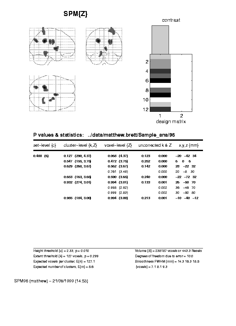
Here is some output from an analysis in SPM96. This analysis will provide the example data for the explanations below:
This is a single subject PET analysis, with covariates only, using proportional scaling and all the usual SPM96 defaults. I have selected the 12 files for this subject in scan order (1 to 12); for the covariate I entered the numbers for Task Difficulty that you see in the tables below. I asked for a single contrast, which was '1' (see below). If you would like to, and you have SPM96 (or 99) you can reproduce the analysis. You will need to download the image files, and unpack them to a suitable directory (see the http://imaging.mrc-cbu.cam.ac.uk/scripts/statstalk.m file for instructions).
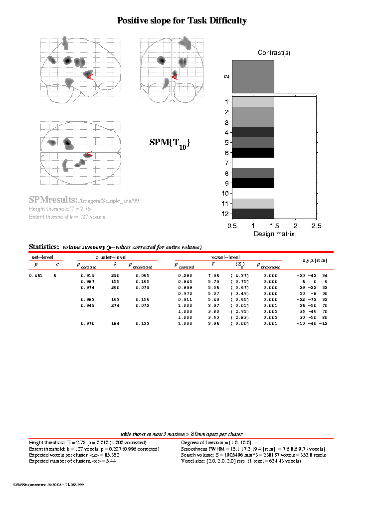
Here is the same analysis performed in SPM99:
In this tutorial, I hope to explain exactly how the Z scores from these tables have been calculated. The Z scores are the numbers in the centre of the tables that are in brackets; for SPM96 the Z scores are in a column labelled 'voxel-level{Z}', and for SPM99, they are under the 'voxel-level' heading, in the 'Z=' column. I will also try to explain the meaning of the 'Design matrix' graphic in the top right hand corner of these pages, and the 'Contrast' graphic above it.
Step one: getting the data from the images
In order to do the statistics for a certain voxel, SPM needs to obtain the data for that voxel, for each of the scans in the analysis. You can see how SPM does this inhttp://imaging.mrc-cbu.cam.ac.uk/scripts/statstalk.m. In essence, it finds which of the numbers that comprise an image corresponds to the voxel required, and extracts that number into matlab, for each scan. We will first obtain the data for the top voxel in the analyses above, that is at coordinates x = -20, y = -42 z = 34.
Step two: getting the data ready to analyse
After getting the data, a few more processing steps may be required. The next two sections explain the processing that has been done for these data. To avoid information overload, you may wish to take this processing on trust for now, and skip on the next main section, Statistics: the simplest case - a regression.
Global image signal
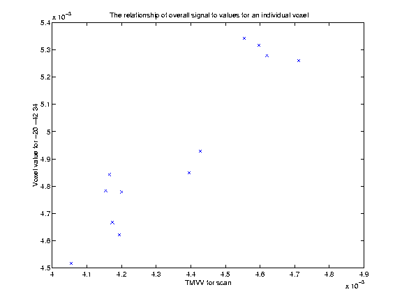
An important step in this analysis will be adjusting the data for the effect of global image signal. By global image signal, I mean the overall magnitude of all the VVs in an image. A large part of the variation of VVs between scans is explained by the overall amount of signal in the scan from which the VV has come. In the case of PET, the amount of signal in the scan is dictated by the amount of radioactivity that has reached the head, and this in turn is influenced by several factors, including the speed of blood circulation from the arm to the heart, and the amount of radioactivity injected. Thus, for a scan where a large amount of radioactivity has reached the head, all the VVs in the brain are likely to be higher than for the equivalent voxel from a scan where less radioactivity is present. SPM attempts to estimate this global signal by using a Thresholded Mean Voxel Value (TMVV). To calculate the TMVV, it does a two-pass mean of the values in the image. First it takes all the numbers that make up the image, and calculates the average of all these numbers. For the first scan in the example dataset, this mean is 0.0038. It then divides this mean value by 8, to give a threshold, on the basis that any voxel with a value this low is likely to be outside the brain. It then calculates the mean of all the VVs that are greater than this threshold. For our first scan, the threshold is 0.0038/8, 415717 of the 510340 voxels in the scan are above this threshold, and the mean of these 415717 values is 0.0046. The code for these calculations is in http://imaging.mrc-cbu.cam.ac.uk/scripts/statstalk.m. Below is a graph of the VVs from the (-20 -42 34) voxel, plotted against the TMVV for the scan from which the voxel came:
As you can see from the figure, higher TMVV values for the scan are associated with higher voxel values in our voxel of interest. For the reasons we discussed above, this is not very surprising, and indeed, the same relationship hold true right across the brain; so that the global signal / TMVV for a scan is a strong predictor of the values for the voxels from that scan. The factors that influence this overall level of signal, which we enumerated above, are usually unrelated to our experimental design; we will therefore need to try and remove this effect if we wish to see the smaller effects that our experiment has caused in our data. One simple way of doing this is to divide each VV by the TMVV for the scan from which it comes. The new VVs are therefore ratios of the value for this voxel to the overall average VV for the scan, where this average is calculated across all the voxels in the brain. For the example voxel, the value for the first scan was 0.053, and the TMVV was 0.046. The new VV, after proportional scaling, is 0.053/0.046 = 1.15.
Grand mean scaling
Grand mean scaling is another common manipulation to the voxel data before it goes into the analysis. Grand mean scaling is used to try and scale the VVs to give them a more readily comprehensible interpretation. For example, the VVs for our chosen voxel are in more or less arbitrary units, given to us by the PET scanner. As you can see from the figure above, for our example voxel the values range from about 0.0045 to 0.0054. The range of these values has no interesting physiological interpretation, so that can be helpful to mutliply the values by a scalefactor so that the units are easier to interpret. The choice of this scalefactor is in itself rather arbitrary. In activation PET studies, it is often assumed that the average blood flow across the whole brain, and across all the scans in the analysis, will have been about 50 mls of blood / 100 mls of brain tissue /min, which is a physiologically plausible value. We can adjust our arbitrary units by multiplying by a scale factor that makes the average of all the TMVVs (one per scan) to be equal to 50. This means that the units for the VVs will be something near to a guessed blood flow value, although this guess is extremely approximate. In our case, we have already proportionally scaled our images, so, by definition, the TMVV of all our scans is 1, and the mean of these values is also one. So to GM scale our VVs, we merely multiply them all by 50. In this simple case, with one subject, where all the scans are being scaled by the same factor, the GM scaling has no effect on the statistics; it only changes the units of the data.
Statistics: the simplest case - a regression
Our example SPM analysis is a simple regression. For our example we have 12 scans for a single subject, and we have recorded a covariate, task difficulty (TD) for each scan. Our hypothesis is that increasing TD causes an increase in VVs. Here are the VVs for our example voxel (-20 -42 34), with the TD values, for each scan:
Scan no |
Voxel 1 |
Task difficulty |
1 |
57.84 |
5 |
2 |
57.58 |
4 |
3 |
57.14 |
4 |
4 |
55.15 |
2 |
5 |
55.90 |
3 |
6 |
55.67 |
1 |
7 |
58.14 |
6 |
8 |
55.82 |
3 |
9 |
55.10 |
1 |
10 |
58.65 |
6 |
11 |
56.89 |
5 |
12 |
55.69 |
2 |
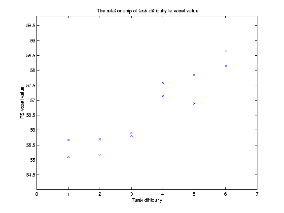
The graph below shows a plot of the VVs against TD:
Our hypothesis is that increasing TD is associated with increasing VVs. We might be more bold, and say that we believe that there is a linear relationship of TD to VV. This is the same as saying that we think that the relationship of TD to the VVs can be expressed as a straight line on our graph above, which can be defined by its intercept on the Y axis and its slope. Let us for the moment guess that this line has an intercept at y=55, and a slope of 0.5 VV units per unit increment in TD. This gives us a line (see below). but is it the best line? One way of assessing whether a line is a good fit to the data is by looking at the mean squared difference between the actual data points, and the corresponding points as predicted by the line. On the graph below, I have plotted the data, my guess at the best line, and vertical lines showing the distance of the data points from the points predicted by the line:
The distances of the data points from the line are termed residuals, because they are the data that remains after the linear relationship has been taken into account. If we square each of these residuals, they will now all be positive, and will be larger the further away the point is from the line. The average of these squared residuals is a measure of how well, on average, the line fits the data; the smaller this mean squared residual, the better the line can be said to fit the data. [In fact, for reasons that are not worth going into here, we do not use the simple number of observations in calculating this average, but the number of available degrees of freedom (df). In our case the df are simply the number of observations minus 2 - i.e 10]. For our line, we can calculate that the mean squared residual is 0.31.
We now have a metric for deciding how well our line fits the data. If we can find a line with the smallest possible mean squared residual, this line will be the best fitting line, in the sense that it results in the least squares of the residuals. In order to work out our least squares fit for the line, we need to formalise our problem a little.
So, let us express our hypothesis in more formal terms. We believe that there is a linear relationship of TD to VVs. This means that we have a model for our data, which can be expressed thus:
Y(j) = beta * x(j) + c + E(j)
where:
j indexes the scans from 1 to 12;
Y is the data for each scan at this voxel (the response variable);
beta is the slope of the line, which has yet to be worked out;
x is the TD for each scan (our predictor variable);
c is the y intercept of the line, which has yet to be worked out;
E is the remaining error, or residual, for each scan.
Returning to our table therefore, the data in column 2 (Voxel 1) are the VVs for each scan, Y(j). Y(1) is therefore 57.84, and so on. Similarly the data in column 3 (Task difficulty) are the TD scores for each scan, x(j).
This is the statistical formula for a simple regression. The formula states that we believe that our data are made up of a linear effect of TD (beta * x(j) + c), plus some random fluctuations, that we cannot explain (E(j)).
In order to work out our best fitting line, we have to do a little more reformulation. It turns out that the problem can be very simply solved if we can re-express our formula in terms of matrices. Using matrices here has huge advantages; it will make our calculations much more straightforward to perform, and will also allow us to use the same maths for a huge number of different regression problems, as we will begin to see later on.
From model to matrices
SPM, and indeed almost all statistical techniques, work with matrices. In this section, we will rephrase our simple model in terms of matrices. If you don't know the first thing about matrices, or have forgotten, then have a look at my matrix refresher page, which is a little pdf document (see the online reading page if you have trouble reading this format).So, we wish to rephrase our data and model in terms of matrices. This is easy for Y(j) and x(j), which are already both vectors. But how about c, the constant? We can get round this by adding a column to our table, Constant variable (cv), which contains only ones.
Scan no |
Voxel 1 |
Task difficulty |
Constant variable |
1 |
57.84 |
5 |
1 |
2 |
57.58 |
4 |
1 |
3 |
57.14 |
4 |
1 |
4 |
55.15 |
2 |
1 |
5 |
55.90 |
3 |
1 |
6 |
55.67 |
1 |
1 |
7 |
58.14 |
6 |
1 |
8 |
55.82 |
3 |
1 |
9 |
55.10 |
1 |
1 |
10 |
58.65 |
6 |
1 |
11 |
56.89 |
5 |
1 |
12 |
55.69 |
2 |
1 |
This gives a model:
Y(j) = beta * x(j) + c * cv(j)+ E(j)
Which, because cv(j) is always 1, is exactly the same as:
Y(j) = beta * x(j) + c + E(j)
i.e. our original model.
Now we can rephrase our model in terms of matrices:
Y = X * B + E
(note that Y, X, B and E, the matrices, are now in bold)
Where Y is the data matrix:
57.84 |
57.58 |
57.14 |
55.15 |
55.90 |
55.67 |
58.14 |
55.82 |
55.10 |
58.65 |
56.89 |
55.69 |
X is the design matrix:
5 |
1 |
4 |
1 |
4 |
1 |
2 |
1 |
3 |
1 |
1 |
1 |
6 |
1 |
3 |
1 |
1 |
1 |
6 |
1 |
5 |
1 |
2 |
1 |
B is the parameter matrix:
Beta |
C |
And E is the error matrix, with one column and 12 rows:
remaining error for scan 1 |
remaining error for scan 2 |
... |
remaining error for scan 12 |
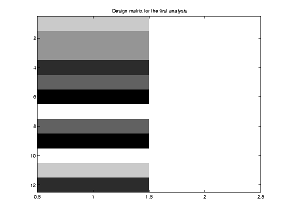
This design matrix is precisely the design matrix used by SPM. As you can see from the analysis printouts, SPM displays this design matrix to you graphically, scaling each column so that the most negative number in the column will be nearest to black, and the most positive will be nearest to white. For example, the first column in the design matrix above varies from one to six. In the SPM display for this design matrix, for the first column, ones will be shown as black, sixes as white, and the rest as intermediate greys. The design matrix above will therefore look like the figure below. As you would expect, in the first column of the picture, the sixth and ninth rows in the picture are black, corresponding to the ones in the design matrix, and rows seven and ten are white corresponding to the sixes in the design matrix.
Because of the way matrix multiplication works, our matrix model (Y=X*B+E) is mathematically the same as our previous version of the formula, i.e.:
Y(j) = beta * x(j) + c + E(j)
Thus the top row of Y (Y(1)) is:
x(1)* beta + cv(1) * c + E(1) ( = 5 * beta + c + error-for-scan-1),
the second row of Y is:
x(2)* beta + cv(2) * c + E(2) ( = 4 * beta + C + error-for-scan-2),
and so on.
The matrix formulation makes it very easy to find our least square fit for the line. It can be performed in one line of matlab code:
B = inv(X)*Y
where
inv(X)
is the inverse of the design matrix. Please see Andrew Holmes' chapter in the SPM course notes for the derivation of the maths. We now have a matrixBthat contains the least squares estimates of our parameters:
0.64 |
54.39 |
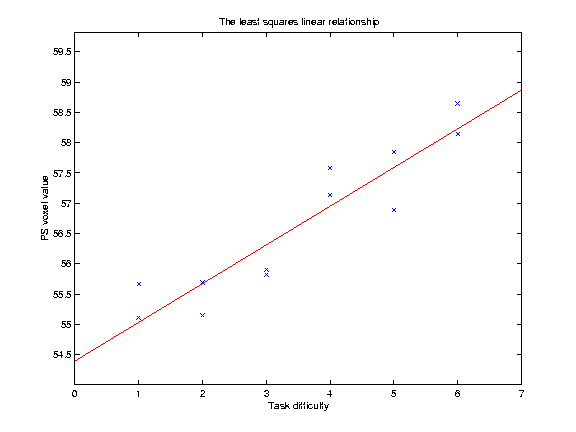
where the first element of B, 0.64, is the slope of the line, beta, and the second element of B, 54.39, is the y intercept, c.
Below is a plot of the data with the least squares fitting line:
We can work out the remaining errors E by:
E = Y - X * B
which is the same as saying
E(1) = Y(1) - beta * x(1) + c,
E(2) = Y(2) - beta * x(2) + c, etc.
which are the same as the distances of the voxel data values from the values predicted by our least squares fitting line. Remember that the mean squared residual for my guess at the line was 0.31; as we would expect, the mean squared residual for the best fitting line is indeed less, at 0.23.
t statistics and contrasts
Our original reason for looking at the slope of the data against TD was because we thought VVs would increase linearly with increasing TD. We can assess whether this was the case, because, if so, there will be a positive slope linking TD with our VVs. We test this against the null hypothesis. The null hypothesis is that there is no relationship between TD and the voxel data. On the null hypothesis, beta, the slope of the line, will not be significantly different from zero. We can test this by making a t statistic, where the t statistic is:
beta / (the standard error of the slope)
(this test is equivalent to a test for a non-zero correlation, between TD and the VVs). The standard error can be worked out from the original analysis of variance, using the remaining error, matrix E above (see http://imaging.mrc-cbu.cam.ac.uk/scripts/statstalk.m for the code, and Andrew Holmes' chapter in the SPM course notes for more detail). This t statistic will be large and positive if the slope is significantly greater than 0, and large and negative if the slope is significantly less than 0.
In this case, it is very simple to obtain the numerator of the t statistic, which is "beta". However, as we will see below, sometimes the design matrix has many columns, and our hypothesized effect is more complicated. In these cases, it is useful to express our hypothesis with a more general mechanism, called a "contrast". This very general mechanism is used by SPM to express hypotheses about the effects defined the the design matrix. For example, here we are looking at the effect of TD.
So, to get the numerator of the t statistic for TD, we can use a contrast weights vector. I will refer to this contrast weights vector simply as a "contrast" in what follows. The contrast is a matrix that, when multiplied by B, gives you the numerator of the t statistic. Here, the matrix would be (1 0), because:
1 |
0 |
*
Beta |
C |
= beta
In fact, SPM will conceal the constant from you, by terming it an 'effect of no interest', so effectively your B becomes:
(beta)
and your contrast is (1). This is how you specify a contrast for a single covariate-of-interest in SPM. As the http://imaging.mrc-cbu.cam.ac.uk/scripts/statstalk.m file shows, a few lines of matlab code will generate the t value for the example voxel and contrast, which is 7.96. Reassuringly, this is the value that SPM99 displays for this voxel in the printout above.
SPM will do the calculation above for every voxel in the brain, and thus, for every voxel, there will be a separate beta. This contrast can provide a t statistic for every voxel, that is positive where the best fitting line has a positive slope and negative where it has a negative slope.
A short note on hypothesis testing
The t statistic we have is an example of an hypothesis test. The t statistic is testing the null hypothesis, that there is no linear relationship of TD with the VVs; if there is no linear relationship, then the slope relating the two should be zero. We have only a few observations (12) to estimate the slope, so our measurement of the slope will be subject to error. Thus our question becomes; given the error in our observations, could this estimate we have of the slope (beta) have come about by chance, even if the null hypothesis is true? Conversely, is beta too large for this to be plausible? So, the t statistic is our least squares estimate of the slope, divided by a measure of the error of the slope, and is therefore an index of how far the slope differs from zero, given the error. We know the distribution of the t statistic, so, we can say that, by chance, with 10 degrees of freedom, a t statistic of 7.96 or greater occurs 0.0006 percent of the time, if the null hypothesis is true (the p value is 0.000006). This seems pretty unlikely; however, we must remember that in an SPM map of statistics we have a severe multiple comparison problem - see the random fields tutorial for more detail.
From t statistics to Z scores
After calculating the t statistic, SPM converts the t statistics to Z scores. Z scores are a way that SPM uses to display and analyse the p values from the t statistics. The Z scores are the numbers from the unit normal distribution (mean 0 sd/variance 1) that would give the same p value as the t statistic. For example, let us say we had a t value for one voxel that was -2.76. For the analysis above there are 10 degrees of freedom (df). That gives a one-tailed (lower tail) p value of 0.01. This p value should be interpreted as saying that 1% of the time by chance, with 10 df, I would find a t valueless than or equal to-2.76, and this is the same as saying that 1% of the area of the t distribution, with 10 df, lies below -2.76. The equivalent Z score is -2.33, because 1% of the normal distribution lies below -2.33. By the same logic, with a t value of +2.76, my p value will be 0.99 - i.e. 99% of the time I would expect to find a t value less than or equal to 2.76 (and 1% of the time I will find a higher p value). A p value of 0.99 gives me a Z score of +2.33 (99% of the normal distribution lies below 2.33).If you then ask SPM96 to show you a picture of the Z statistics, thresholded at a Z score of 2.33, then it will only show you Z scores more positive than 2.33, which would be exactly the same as showing you any t statistics more positive than 2.76 in this analysis. Conversely if you want to see voxels with slopes significantly less than 0, you would have to apply the contrast (-1), so that now negative betas become positive, and therefore the negative t statistics become positive. You would then again ask SPM96 to show you Z scores of greater than 2.33.
SPM99 works with t statistics rather than Z scores, so to see the same set of voxels you would have to threshold at t = 2.76.
More than one covariate
The same principle for the statistics easily extends to the situation where you think that two variables might explain some of the voxel data. For example, let us imagine that it is a visual task that the subjects are doing in the scanner, and that along with task difficulty (TD), you have recorded the presentation rate of visual stimuli (PR) which is independent of TD. You might want to put in PR because you were interested in its effect on blood flow, or because you thought it might explain some data variance, and thus improve your model and your estimate of the effect of TD.
This gives you the model:
Y(j) = beta(TD) * x(TD)(j) + beta(PR)* x(PR)(j) + c + E(j)
where beta(TD) is the slope relating your data to TD, x(TD)(j) is the task difficulty score for scan j, beta(PR) is the slope relating your data to PR, and x(PR)(j) is the presentation rate during scan j.
The table of example data might now look like this:
Scan no |
Voxel 1 |
Task difficulty |
PR |
1 |
57.84 |
5 |
1 |
2 |
57.58 |
4 |
2 |
3 |
57.14 |
4 |
3 |
4 |
55.15 |
2 |
4 |
5 |
55.90 |
3 |
5 |
6 |
55.67 |
1 |
6 |
7 |
58.14 |
6 |
7 |
8 |
55.82 |
3 |
8 |
9 |
55.10 |
1 |
9 |
10 |
58.65 |
6 |
10 |
11 |
56.89 |
5 |
11 |
12 |
55.69 |
2 |
12 |
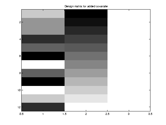
And the design matrix will be:
5 |
1 |
1 |
4 |
2 |
1 |
4 |
3 |
1 |
2 |
4 |
1 |
3 |
5 |
1 |
1 |
6 |
1 |
6 |
7 |
1 |
3 |
8 |
1 |
1 |
9 |
1 |
6 |
10 |
1 |
5 |
11 |
1 |
2 |
12 |
1 |
Which will be displayed in SPM as:
The same procedure as we used before will give you least squares fits for beta(TD), beta(PR) and c, and the parameter matrix B is:
Beta(TD) |
Beta(PR) |
C |
Again, SPM conceals the last parameter from you as a covariate of no interest, and thus, the effective B is:
Beta(TD) |
Beta(PR) |
If you want a t statistic to assess how positive the slope of TD is, having taken into account the effect of PR, you use the contrast:
(1 0)
giving the top half of your t statistic:
beta(TD)
and you then proceed as before. Similarly, if you want a t statistic assessing how positive the slope of PR is, against the data, having taken into account the effect of TD, you use the contrast:
(0 1)
giving the top half of your t statistic:
beta(PR).
Adding conditions: the General Linear Model
The situation becomes a little more complex when you enter conditions into your model. So far the analyses have been regressions. You can use the same principles to look at condition effects, using the General Linear Model. The general linear model allows you to phrase an analysis of variance with condition or group effects in terms of a multiple regression. This is a standard statistical technique which is used in virtually all commercial statistics packages - SPSS, SAS etc.This is how it works in SPM. Let us say we have a new experiment, now with 12 scans, 6 in the rest condition (R), and 6 in the activation condition (A). We can phrase our model in terms of a linear regression:
Y(j) = beta(R) * x(R)(j) + beta(A)* x(A)(j) + E(j)
Here again beta(R), beta(A) are constants yet to be worked out, and x(R), x(A) are new 'dummy' variables which we will have to make up to give the correct analysis. It is this use of dummy variables that allows the general linear model to phrase the conditions ANOVA in terms of a multiple regression. One way to create these variables, and the way that SPM chooses, is to make x(R) to be a variable, for each scan, that will be 1 if the scan is a rest scan, and 0 if it is not a rest scan. Similarly x(A) is a variable, for each scan, that will be 1 if the scan is an activation scan, and 0 if it is not an activation scan. So, these dummy variables are indicator variables, where the variable values indicate whether or not the particular scan is in a particular condition; thus the X(A) variable indicates whether or not the scan is in the activation condition. In order to get a least squares fit, the parameter beta(R) must be the mean for the VVs in the rest condition, and beta(A) must be the mean for the VVs in the activation condition.
So, if the first 6 scans are rest, and the last 6 scans are activation, the design matrix will be:
1 |
0 |
1 |
0 |
1 |
0 |
1 |
0 |
1 |
0 |
1 |
0 |
0 |
1 |
0 |
1 |
0 |
1 |
0 |
1 |
0 |
1 |
0 |
1 |
Which will be displayed in SPM as:
So we have, after our ANOVA, the following B:
Beta(R) |
Beta(A) |
We want to look for voxels which have significantly greater values in the A than the R condition. Our t statistic is now:
(mean for A scans) - (mean for R scans) / SE
which is the same as:
( (-1 1) * B ) / SE
So the contrast for this comparison is (-1 1). Conversely, to look for voxels which have significantly greater values in the R than the A condition, the contrast is (1 -1), giving a t of
mean(R) - mean(A) / SE
The end
I hope that it is at least in principle clear how one would extend this to include conditions and covariates, and having more than one subject, but in any case maybe this is a start...Please email any comments or suggestions, and I'll try and include them.
Many thanks in particular to Andrew Holmes, Jon Simons and Thomasin Andrews for their helpful comments on various drafts of this page. Of course any errors are all mine...
MatthewBrett 19/8/99 (FB)
