Autonomous Driving Steering Control
目录
A . 基于道路几何模型的方法
B . 基于运动学模型的算法(以mpc为例)
A . 基于道路几何模型的方法
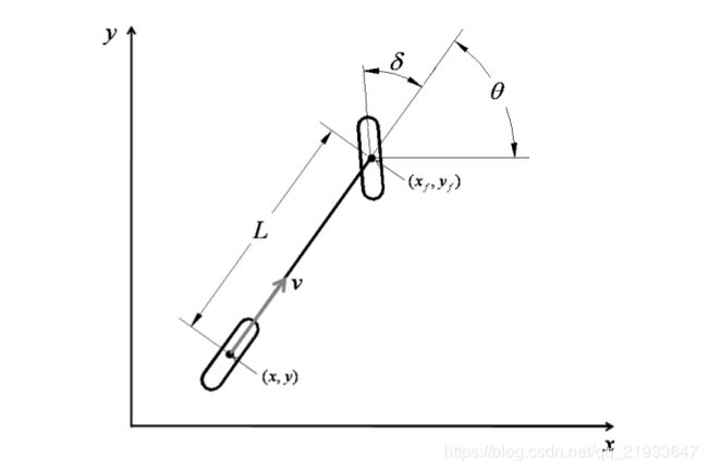
A.1 几何自行车模型

二自由度自行车模型 : 前轮转向,后轮绕旋转中心做圆周运动,转向半径和转向前轮偏角满足如下关系:
![]() (1)
(1)
L为车辆轴距(广义用法为等效轴距),delta 为前轮转角, R后轮中心(广义用法为等效后轮中心)转弯半径。
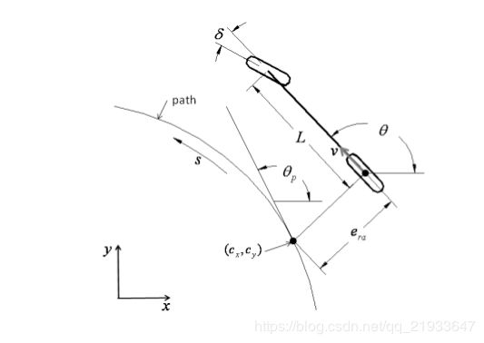
A.2 pure pursuit 算法
算法核心原理如下图所示:

算法原理阐述 : 给定参考路径path , 在参考路径上离车辆等效后轴中心一个预瞄距离的点 ![]() , 路径的航向与车辆的航向偏差值为
, 路径的航向与车辆的航向偏差值为 ,转弯半径、航向偏差和预瞄距离之间满足如下关系:
![]() -------------->
--------------> ![]() (2)
(2)
结合A.1二自由度假设(将式(1) 带入式(2))得到前轮偏角(方向盘转角)的计算方法:
![]() (3)
(3)
实际应用时,往往需要加预处理或后处理(二者往往选其一), 常用的预处理(误差平滑)或后处理(输出角度平滑)方法为中值滤波或均值滤波。
参考代码地址(后面方法也参考该代码): https://github.com/AtsushiSakai/PythonRobotics
代码示例:
"""

Path tracking simulation with pure pursuit steering control and PID speed control.


"""
import numpy as np
import math
import matplotlib.pyplot as plt

k = 0.1  # look forward gain
Lfc = 1.0  # look-ahead distance
Kp = 1.0  # speed propotional gain
dt = 0.1  # [s]
L = 2.9  # [m] wheel base of vehicle


show_animation = True


class State:

    def __init__(self, x=0.0, y=0.0, yaw=0.0, v=0.0):
        self.x = x
        self.y = y
        self.yaw = yaw
        self.v = v


def update(state, a, delta):

    state.x = state.x + state.v * math.cos(state.yaw) * dt
    state.y = state.y + state.v * math.sin(state.yaw) * dt
    state.yaw = state.yaw + state.v / L * math.tan(delta) * dt
    state.v = state.v + a * dt

    return state


def PIDControl(target, current):
    a = Kp * (target - current)

    return a


def pure_pursuit_control(state, cx, cy, pind):

    ind = calc_target_index(state, cx, cy)

    if pind >= ind:
        ind = pind

    if ind < len(cx):
        tx = cx[ind]
        ty = cy[ind]
    else:
        tx = cx[-1]
        ty = cy[-1]
        ind = len(cx) - 1

    alpha = math.atan2(ty - state.y, tx - state.x) - state.yaw

    if state.v < 0:  # back
        alpha = math.pi - alpha

    Lf = k * state.v + Lfc

    delta = math.atan2(2.0 * L * math.sin(alpha) / Lf, 1.0)

    return delta, ind


def calc_target_index(state, cx, cy):

    # search nearest point index
    dx = [state.x - icx for icx in cx]
    dy = [state.y - icy for icy in cy]
    d = [abs(math.sqrt(idx ** 2 + idy ** 2)) for (idx, idy) in zip(dx, dy)]
    ind = d.index(min(d))
    L = 0.0

    Lf = k * state.v + Lfc

    # search look ahead target point index
    while Lf > L and (ind + 1) < len(cx):
        dx = cx[ind + 1] - cx[ind]
        dy = cx[ind + 1] - cx[ind]
        L += math.sqrt(dx ** 2 + dy ** 2)
        ind += 1

    return ind


def main():
    #  target course
    cx = np.arange(0, 50, 0.1)
    cy = [math.sin(ix / 5.0) * ix / 2.0 for ix in cx]

    target_speed = 10.0 / 3.6  # [m/s]

    T = 100.0  # max simulation time

    # initial state
    state = State(x=-0.0, y=-3.0, yaw=0.0, v=0.0)

    lastIndex = len(cx) - 1
    time = 0.0
    x = [state.x]
    y = [state.y]
    yaw = [state.yaw]
    v = [state.v]
    t = [0.0]
    target_ind = calc_target_index(state, cx, cy)

    while T >= time and lastIndex > target_ind:
        ai = PIDControl(target_speed, state.v)
        di, target_ind = pure_pursuit_control(state, cx, cy, target_ind)
        state = update(state, ai, di)

        time = time + dt

        x.append(state.x)
        y.append(state.y)
        yaw.append(state.yaw)
        v.append(state.v)
        t.append(time)

        if show_animation:
            plt.cla()
            plt.plot(cx, cy, ".r", label="course")
            plt.plot(x, y, "-b", label="trajectory")
            plt.plot(cx[target_ind], cy[target_ind], "xg", label="target")
            plt.axis("equal")
            plt.grid(True)
            plt.title("Speed[km/h]:" + str(state.v * 3.6)[:4])
            plt.pause(0.001)

    # Test
    assert lastIndex >= target_ind, "Cannot goal"

    if show_animation:
        plt.plot(cx, cy, ".r", label="course")
        plt.plot(x, y, "-b", label="trajectory")
        plt.legend()
        plt.xlabel("x[m]")
        plt.ylabel("y[m]")
        plt.axis("equal")
        plt.grid(True)

        flg, ax = plt.subplots(1)
        plt.plot(t, [iv * 3.6 for iv in v], "-r")
        plt.xlabel("Time[s]")
        plt.ylabel("Speed[km/h]")
        plt.grid(True)
        plt.show()


if __name__ == '__main__':
    print("Pure pursuit path tracking simulation start")
    main()
A.3 基于前轮反馈的Stanley算法
算法核心原理示意图 :

算法原理阐述 : 给定参考路径path ,在路径上寻找离前轮中心最近点![]() , 计算该点与前轮中心的横向偏差
, 计算该点与前轮中心的横向偏差![]() 和 车身的航向偏差
和 车身的航向偏差![]() , 其前轮方向盘转角(前轮偏角) 为 :
, 其前轮方向盘转角(前轮偏角) 为 :
![]() (4)
(4)
v为车速,k为比例因子(可调节参数)。实际应用时,需要对路径做平滑的处理。
代码示例:
"""

Path tracking simulation with Stanley steering control and PID speed control.

"""
from __future__ import division, print_function

import sys

sys.path.append("../../PathPlanning/CubicSpline/")

import matplotlib.pyplot as plt
import numpy as np

import cubic_spline_planner

k = 0.5  # control gain
Kp = 1.0  # speed propotional gain
dt = 0.1  # [s] time difference
L = 2.9  # [m] Wheel base of vehicle
max_steer = np.radians(30.0)  # [rad] max steering angle

show_animation = True


class State(object):
    """
    Class representing the state of a vehicle.

    :param x: (float) x-coordinate
    :param y: (float) y-coordinate
    :param yaw: (float) yaw angle
    :param v: (float) speed
    """

    def __init__(self, x=0.0, y=0.0, yaw=0.0, v=0.0):
        """Instantiate the object."""
        super(State, self).__init__()
        self.x = x
        self.y = y
        self.yaw = yaw
        self.v = v

    def update(self, acceleration, delta):
        """
        Update the state of the vehicle.

        Stanley Control uses bicycle model.

        :param acceleration: (float) Acceleration
        :param delta: (float) Steering
        """
        delta = np.clip(delta, -max_steer, max_steer)

        self.x += self.v * np.cos(self.yaw) * dt
        self.y += self.v * np.sin(self.yaw) * dt
        self.yaw += self.v / L * np.tan(delta) * dt
        self.yaw = normalize_angle(self.yaw)
        self.v += acceleration * dt


def pid_control(target, current):
    """
    Proportional control for the speed.

    :param target: (float)
    :param current: (float)
    :return: (float)
    """
    return Kp * (target - current)


def stanley_control(state, cx, cy, cyaw, last_target_idx):
    """
    Stanley steering control.

    :param state: (State object)
    :param cx: ([float])
    :param cy: ([float])
    :param cyaw: ([float])
    :param last_target_idx: (int)
    :return: (float, int)
    """
    current_target_idx, error_front_axle = calc_target_index(state, cx, cy)

    if last_target_idx >= current_target_idx:
        current_target_idx = last_target_idx

    # theta_e corrects the heading error
    theta_e = normalize_angle(cyaw[current_target_idx] - state.yaw)
    # theta_d corrects the cross track error
    theta_d = np.arctan2(k * error_front_axle, state.v)
    # Steering control
    delta = theta_e + theta_d

    return delta, current_target_idx


def normalize_angle(angle):
    """
    Normalize an angle to [-pi, pi].

    :param angle: (float)
    :return: (float) Angle in radian in [-pi, pi]
    """
    while angle > np.pi:
        angle -= 2.0 * np.pi

    while angle < -np.pi:
        angle += 2.0 * np.pi

    return angle


def calc_target_index(state, cx, cy):
    """
    Compute index in the trajectory list of the target.

    :param state: (State object)
    :param cx: [float]
    :param cy: [float]
    :return: (int, float)
    """
    # Calc front axle position
    fx = state.x + L * np.cos(state.yaw)
    fy = state.y + L * np.sin(state.yaw)

    # Search nearest point index
    dx = [fx - icx for icx in cx]
    dy = [fy - icy for icy in cy]
    d = [np.sqrt(idx ** 2 + idy ** 2) for (idx, idy) in zip(dx, dy)]
    error_front_axle = min(d)
    target_idx = d.index(error_front_axle)

    target_yaw = normalize_angle(np.arctan2(fy - cy[target_idx], fx - cx[target_idx]) - state.yaw)
    if target_yaw > 0.0:
        error_front_axle = - error_front_axle

    return target_idx, error_front_axle


def main():
    """Plot an example of Stanley steering control on a cubic spline."""
    #  target course
    ax = [0.0, 100.0, 100.0, 50.0, 60.0]
    ay = [0.0, 0.0, -30.0, -20.0, 0.0]

    cx, cy, cyaw, ck, s = cubic_spline_planner.calc_spline_course(
        ax, ay, ds=0.1)

    target_speed = 30.0 / 3.6  # [m/s]

    max_simulation_time = 100.0

    # Initial state
    state = State(x=-0.0, y=5.0, yaw=np.radians(20.0), v=0.0)

    last_idx = len(cx) - 1
    time = 0.0
    x = [state.x]
    y = [state.y]
    yaw = [state.yaw]
    v = [state.v]
    t = [0.0]
    target_idx, _ = calc_target_index(state, cx, cy)

    while max_simulation_time >= time and last_idx > target_idx:
        ai = pid_control(target_speed, state.v)
        di, target_idx = stanley_control(state, cx, cy, cyaw, target_idx)
        state.update(ai, di)

        time += dt

        x.append(state.x)
        y.append(state.y)
        yaw.append(state.yaw)
        v.append(state.v)
        t.append(time)

        if show_animation:
            plt.cla()
            plt.plot(cx, cy, ".r", label="course")
            plt.plot(x, y, "-b", label="trajectory")
            plt.plot(cx[target_idx], cy[target_idx], "xg", label="target")
            plt.axis("equal")
            plt.grid(True)
            plt.title("Speed[km/h]:" + str(state.v * 3.6)[:4])
            plt.pause(0.001)

    # Test
    assert last_idx >= target_idx, "Cannot reach goal"

    if show_animation:
        plt.plot(cx, cy, ".r", label="course")
        plt.plot(x, y, "-b", label="trajectory")
        plt.legend()
        plt.xlabel("x[m]")
        plt.ylabel("y[m]")
        plt.axis("equal")
        plt.grid(True)

        flg, ax = plt.subplots(1)
        plt.plot(t, [iv * 3.6 for iv in v], "-r")
        plt.xlabel("Time[s]")
        plt.ylabel("Speed[km/h]")
        plt.grid(True)
        plt.show()


if __name__ == '__main__':
    main()
B . 基于运动学模型的算法(以mpc为例)
B1. 运动学模型
1. 笛卡尔坐标系下的运动学模型
非完整性约束(nonholonomic constraint,对于轮式车而言非完整性约速为车轮垂向速度为0)的运动学模型 ,其示意图如下所示:
根据非完整性约束,得到微分方程:
![]() (5)
(5)
![]() (6)
(6)
根据车辆几何信息![]() , 结合式(5) 和(6)可以得到:
, 结合式(5) 和(6)可以得到:
![]() (7)
(7)
结合式子(6) 、(7)可以得到车辆的运动学方程为:
(8)
2. 道路坐标系(Frenet)下的运动学模型(CMU 论文里有些描述存在错误)
道路坐标系下运动学模型经典表述为误差模型:
航向误差: ![]()
曲率: ![]()
沿道路弧长的一阶导(match point 在路径上的平移速度): ![]()
横向偏差一阶导: ![]()
综上所述4个公式得Frenet坐标系下的运动学模型为:
(9)
温馨提示: 使用该模型时,需要先拟合参考路径的参数方程,拟合方法参考博客(Cubic Spline Interpolation ).
B2. 模型预测控制思想
1. 模型预测控制思想
模型预测控制是一类通过滚动求解带约束优化问题的控制方法,有文献也将其称为滚动优化控制。根据所采用模型的不同,主要包括动态矩阵控(Dynamic Matrix Control, DMC)、模型算法控制(Model Algorithm Control, MAC)和广义预测控制(Generalized Predictive Control, GPC)等。同时,在现代控制理论中所广泛使用的状态空间模型,同样可以应用于模型预测控制中。模型预测控制的一个显著特点就是能方便的处理控制过程中的各种约束,包括系统状态约束、输出约束以及控制量约束等。同时,它还具备鲁棒性好,易于处理非线性系统等优点。
虽然模型预测控制的种类多样,实现方式也有所区别,但都是建立在预测模型、滚动优化和反馈矫正三项基本原理基础上的。
(1)预测模型:预测模型是模型预测控制的基础,主要功能是根据对象的历史信息和未来输入预测系统未来的输出。预测模型的形式没有严格的限定,状态方程、传递函数这类传统的模型都可以作为预测模型。对于线性稳定系统,阶跃响应、脉冲响应这类非参数模型,也可以直接作为预测模型使用。
(2)滚动优化:模型预测控制通过某一性能指标的最优来确定控制作用,但优化不是一次离线进行,而是反复在线进行的,这就是滚动优化的含义,也是模型预测控制区别于传统最优控制的根本点。
(3)反馈校正:为了防止模型失配或者环境干扰引起控制对理想状态的偏离,在新的采样时刻,首先检测对象的实际输出,并利用这一实时信息对基于模型的预测进行修正,然后再进行新的优化。
基于这三个要素,模型预测控制的基本原理可以用图1 来表示。控制过程中,始终存在一条期望轨迹,如图中红色曲线所示。以时刻 k 作为当前时刻,控制器结合当前的测量值和预测模型,预测系统未来一段时域内(也称为预测时域)系统的输出,如图中黄色曲线所示。通过求解满足目标函数以及各种约束的优化问题,得到在控制时域内一系列的控制序列,如图中的矩形波所示,将该控制序列的第一个元素作为受控对象的实际控制量。当来到下一个时刻 k+1 时,重复上述过程,如此滚动的完成一个个带约束的优化问题,实现对被控对象的持续控制。

图 1. MPC 原理示意图
2. 模型预测控制问题描述
/////后续做个专题,简要陈述一下建模,模型精度,densing , 滚动优化求解等问题