Focal Loss for Dense Object Detection（RetinaNet）读书笔记

照例是先翻译，再介绍。

Focal Loss for Dense Object Detection

Abstract

The highest accuracy object detectors to date are based on a two-stage approach popularized by R-CNN, where a classifier is applied to a sparse set of candidate object locations. In contrast, one-stage detectors that are applied over a regular, dense sampling of possible object locations have the potential to be faster and simpler, but have trailed the accuracy of two-stage detectors thus far. In this paper, we investigate why this is the case. We discover that the extreme foreground-background class imbalance encountered during training of dense detectors is the central cause. We propose to address this class imbalance by reshaping the standard cross entropy loss such that it down-weights the loss assigned to well-classified examples. Our novel Focal Loss focuses training on a sparse set of hard examples and prevents the vast number of easy negatives from overwhelming the detector during training. To evaluate the effectiveness of our loss, we design and train a simple dense detector we call RetinaNet. Our results show that when trained with the focal loss, RetinaNet is able to match the speed of previous one-stage detectors while surpassing the accuracy of all existing state-of-the-art two-stage detectors. Code is at: https://github.com/facebookresearch/Detectron

迄今为止，最精确的目标检测器是基于R-CNN推广的两阶段方法，其中分类器应用于稀疏的候选目标位置集。相比之下，在对可能的目标位置进行规则密集采样的基础上应用的一阶段探测器可能更快、更简单，但迄今为止落后于两阶段检测器的精度。在本文中，我们将研究为什么会出现这种情况。我们发现，在检测器的训练过程中所遇到的极端前景、背景类别不平衡，是造成这种现象的主要原因。我们通过修改标准的交叉熵损失，来解决这一类样本不平衡问题，从而降低正确分类样本的损失的权重。我们的原创Focal Loss在一组稀疏的难样本上训练，并有效防止大量负样本影响检测器性能。为了评估损失的有效性，我们设计并训练了一个简单的密集检测器，称为RetinaNet。研究结果表明，当使用Focal Loss训练时，RetinaNet与以往的单阶段检测器速度相当，同时超过了现有最先进的两级检测器的精度。代码位于：https://github.com/facebook research/Detectron

1. Introduction

Current state-of-the-art object detectors are based on a two-stage, proposal-driven mechanism. As popularized in the R-CNN framework [11], the first stage generates a sparse set of candidate object locations and the second stage classifies each candidate location as one of the foreground classes or as background using a convolutional neural network. Through a sequence of advances [10, 28, 20, 14], this two-stage framework consistently achieves top accuracy on the challenging COCO benchmark [21].

Despite the success of two-stage detectors, a natural question to ask is: could a simple one-stage detector achieve similar accuracy? One stage detectors are applied over a regular, dense sampling of object locations, scales, and aspect ratios. Recent work on one-stage detectors, such as YOLO [26, 27] and SSD [22, 9], demonstrates promising results, yielding faster detectors with accuracy within 10- 40% relative to state-of-the-art two-stage methods.

This paper pushes the envelope further: we present a one-stage object detector that, for the first time, matches the state-of-the-art COCO AP of more complex two-stage detectors, such as the Feature Pyramid Network (FPN) [20] or Mask R-CNN [14] variants of Faster R-CNN [28]. To achieve this result, we identify class imbalance during training as the main obstacle impeding one-stage detector from achieving state-of-the-art accuracy and propose a new loss function that eliminates this barrier.

当前最先进的对象检测器基于两阶段的提案驱动机制。正如在R-CNN框架中流行的那样[11]，第一阶段生成稀疏的候选对象位置集，第二阶段使用卷积神经网络将每个候选位置分类为前景之一或背景。通过一系列进展[10，28，20，14]，此两阶段框架始终在具有挑战性的COCO基准测试中实现最高准确性[21]。

尽管两级检测器取得了成功，一个自然的问题是：一个简单的一级检测器能否达到类似的精度？一级检测器在常规密集采样得到的目标位置方面，得到了应用。YOLO [26，27]和SSD [22，9]等一阶段检测器的最新工作令人鼓舞，相对于最新的两级检测器，其可产生精度在10％至40％之内的更快检测器方法。

本文将进一步探讨：我们提出了一种单阶段的目标检测器，它首次与更复杂的两级检测器（例如功能金字塔网络（FPN）或Faster R-CNN [28]、Mask R-CNN [14]）在COCO数据集上准确度相当。为了获得此结果，我们将训练过程中的类别不平衡，确定为阻碍一阶段检测器提高精度的主要障碍，并提出了消除这种障碍的新损失函数。

Class imbalance is addressed in R-CNN-like detectors by a two-stage cascade and sampling heuristics. The proposal stage (e.g., Selective Search [35], EdgeBoxes [39], DeepMask [24, 25], RPN [28]) rapidly narrows down the number of candidate object locations to a small number (e.g., 1-2k), filtering out most background samples. In the second classification stage, sampling heuristics, such as a fixed foreground-to-background ratio (1:3), or online hard example mining (OHEM) [31], are performed to maintain a manageable balance between foreground and background.

类不平衡在类R-CNN检测器中通过两级级联和启发性的采样来解决。建议阶段（例如，选择性搜索[35]、EdgeBoxes[39]、DeepMask[24，25]、RPN[28]）快速地将候选对象位置的数目缩小到一个小数目（例如，1-2k），过滤掉大多数背景样本。在第二个分类阶段，为了在前景和背景之间保持可管理的平衡，执行采样启发，例如固定的前景与背景比（1:3）或在线硬示例挖掘（OHEM）[31]。

In contrast, a one-stage detector must process a much larger set of candidate object locations regularly sampled across an image. In practice this often amounts to enumerating ∼100k locations that densely cover spatial positions, scales, and aspect ratios. While similar sampling heuristics may also be applied, they are inefficient as the training procedure is still dominated by easily classified background examples. This inefficiency is a classic problem in object detection that is typically addressed via techniques such as bootstrapping [33, 29] or hard example mining [37, 8, 31].

相比之下，一级检测器必须处理一组更大的候选对象位置，这些候选对象位置在图像上定期采样。在实践中，这通常相当于枚举密集覆盖空间位置、比例和纵横比的100k个位置。虽然也可以应用类似的抽样启发法，但它们效率低下，因为训练过程仍然由容易分类的背景示例支配。这种效率低下是对象检测中的一个典型问题，通常通过引导（bootstrapping）或硬示例挖掘（hard example mining）等技术来解决。

In this paper, we propose a new loss function that acts as a more effective alternative to previous approaches for dealing with class imbalance. The loss function is a dynamically scaled cross entropy loss, where the scaling factor decays to zero as confidence in the correct class increases, see Figure 1. Intuitively, this scaling factor can automatically down-weight the contribution of easy examples during training and rapidly focus the model on hard examples. Experiments show that our proposed Focal Loss enables us to train a high-accuracy, one-stage detector that significantly outperforms the alternatives of training with the sampling heuristics or hard example mining, the previous state-of-the-art techniques for training one-stage detectors. Finally, we note that the exact form of the focal loss is not crucial, and we show other instantiations can achieve similar results.

在本文中，我们提出一个新的损失函数，作为一个更有效的替代方法来处理类不平衡问题。损失函数是一个动态标度的交叉熵损失，当正确分类的样本置信度增加时，标度因子衰减为零，见图1。直观地说，这个比例因子可以自动降低训练过程中简单示例的权重，并快速地将模型集中在硬示例上。实验表明，我们提出的焦点损失使我们能够训练出一种高精度的单级检测器，其性能明显优于以往训练单级检测器的最新技术，即采样启发式或硬示例挖掘。最后，我们注意到Focal loss的确切形式并不重要，并且其他实例可以获得类似的结果。

To demonstrate the effectiveness of the proposed focal loss, we design a simple one-stage object detector called RetinaNet, named for its dense sampling of object locations in an input image. Its design features an efficient in-network feature pyramid and use of anchor boxes. It draws on a variety of recent ideas from [22, 6, 28, 20]. RetinaNet is efficient and accurate; our best model, based on a ResNet-101- FPN backbone, achieves a COCO test-dev AP of 39.1 while running at 5 fps, surpassing the previously best published single-model results from both one and two-stage detectors, see Figure 2.

为了证明所提出的损失的有效性，我们设计了一种简单的单级目标检测器RetinaNet，该检测器以对输入图像中的目标位置进行密集采样命名。其设计特点是高效的网络特征金字塔和锚的使用。它借鉴了[22，6，28，20]中的最新观点。RetinaNet是高效和准确的；我们的最佳模型，基于ResNet-101-FPN骨干网，在5 fps的速度下运行时，COCO测试开发AP达到39.1，超过了先前发布的单级和两级探测器的最佳单模型结果，见图2。

2. Related Work

Classic Object Detectors: The sliding-window paradigm, in which a classifier is applied on a dense image grid, has a long and rich history. One of the earliest successes is the classic work of LeCun et al. who applied convolutional neural networks to handwritten digit recognition [19, 36]. Viola and Jones [37] used boosted object detectors for face detection, leading to widespread adoption of such models. The introduction of HOG [4] and integral channel features [5] gave rise to effective methods for pedestrian detection. DPMs [8] helped extend dense detectors to more general object categories and had top results on PASCAL [7] for many years. While the sliding-window approach was the leading detection paradigm in classic computer vision, with the resurgence of deep learning [18], two-stage detectors, described next, quickly came to dominate object detection.

经典的目标检测器：滑动窗口模式，在密集的图像网格上应用分类器，具有悠久而丰富的历史。最早的成功之一是LeCun等人的经典著作。他将卷积神经网络应用于手写数字识别[19，36]。Viola和Jones[37]使用增强型目标检测器进行人脸检测，导致了此类模型的广泛采用。HOG[4]和积分通道特征[5]的引入为行人检测提供了有效的方法。DPMs[8]有助于将密集探测器扩展到更一般的物体类别，多年来在PASCAL[7]上取得了最好的结果。虽然滑动窗口方法是经典计算机视觉中的主要检测范式，但随着深度学习的兴起[18]，接下来描述的两级检测器很快就占据了目标检测的主导地位。

Two-stage Detectors: The dominant paradigm in modern object detection is based on a two-stage approach. As pioneered in the Selective Search work [35], the first stage generates a sparse set of candidate proposals that should contain all objects while filtering out the majority of negative locations, and the second stage classifies the proposals into foreground classes / background. R-CNN [11] upgraded the second-stage classifier to a convolutional network yielding large gains in accuracy and ushering in the modern era of object detection. R-CNN was improved over the years, both in terms of speed [15, 10] and by using learned object proposals [6, 24, 28]. Region Proposal Networks (RPN) integrated proposal generation with the second-stage classifier into a single convolution network, forming the Faster RCNN framework [28]. Numerous extensions to this framework have been proposed, e.g. [20, 31, 32, 16, 14].

两级检测器：现代目标检测的主要范式是基于两级方法。正如选择性搜索工作[35]所开创的那样，第一阶段生成一个稀疏的候选方案集，该候选方案集应包含所有对象，同时过滤掉大多数负面样本，第二阶段将方案分类为前景类/背景。R-CNN[11]将第二级分类器升级为卷积网络，在精度上有了很大的提高，并开创了现代的目标检测时代。R-CNN经过多年的发展，在速度[15，10]和对象建议[6，24，28]方面取得了较大的进步。区域建议网络（RPN）将生成建议和第二阶段的分类集成到单个卷积网络中，形成更快的RCNN框架[28]。还有其他工作对该框架提出了许多扩展，例如[20、31、32、16、14]。

One-stage Detectors: OverFeat [30] was one of the first modern one-stage object detector based on deep networks. More recently SSD [22, 9] and YOLO [26, 27] have renewed interest in one-stage methods. These detectors have been tuned for speed but their accuracy trails that of twostage methods. SSD has a 10-20% lower AP, while YOLO focuses on an even more extreme speed/accuracy trade-off. See Figure 2. Recent work showed that two-stage detectors can be made fast simply by reducing input image resolution and the number of proposals, but one-stage methods trailed in accuracy even with a larger compute budget [17]. In contrast, the aim of this work is to understand if one-stage detectors can match or surpass the accuracy of two-stage detectors while running at similar or faster speeds.

单级探测器：OverFeat[30]是第一个基于深度网络的现代单级目标探测器。最近，SSD[22,9]和YOLO[26,27]重新激发了研究者对单阶段方法的兴趣。这些探测器具有较快的速度，但其精度落后于两级方法。SSD的AP降低了10-20%，而YOLO则专注于更极端的速度/精度权衡。见图2。最近的研究表明，只需降低输入图像的分辨率和建议框的数量，就可以快速实现两级检测器，但一级方法在精度方面仍然落后，即使计算预算更大[17]。相比之下，这项工作的目的是了解一级探测器在以相似或更快的速度运行时，是否能够匹配或超过两级探测器的精度。

The design of our RetinaNet detector shares many similarities with previous dense detectors, in particular the concept of ‘anchors’ introduced by RPN [28] and use of features pyramids as in SSD [22] and FPN [20]. We emphasize that our simple detector achieves top results not based on innovations in network design but due to our novel loss.

我们的RetinaNet探测器的设计与以前的密集探测器有许多相似之处，特别是RPN[28]引入的“锚”概念，以及在SSD[22]和FPN[20]中使用金字塔特征。我们强调，我们的简单探测器取得了最好的结果不是基于网络设计的创新，而是由于我们的新损失。

Class Imbalance: Both classic one-stage object detection methods, like boosted detectors [37, 5] and DPMs [8], and more recent methods, like SSD [22], face a large class imbalance during training. These detectors evaluate 104- 105 candidate locations per image but only a few locations contain objects. This imbalance causes two problems: (1) training is inefficient as most locations are easy negatives that contribute no useful learning signal; (2) en masse, the easy negatives can overwhelm training and lead to degenerate models. A common solution is to perform some form of hard negative mining [33, 37, 8, 31, 22] that samples hard examples during training or more complex sampling/reweighing schemes [2]. In contrast, we show that our proposed focal loss naturally handles the class imbalance faced by a one-stage detector and allows us to efficiently train on all examples without sampling and without easy negatives overwhelming the loss and computed gradients.

类不平衡：经典的一级目标检测方法，如增强型检测器[37,5]和DPMs[8]，以及较新的方法，如SSD[22]，在训练过程中都面临着较大的类不平衡。这些探测器评估每个图像104-105个候选位置，但只有少数位置包含对象。这种不平衡导致了两个问题：（1）训练效率低下，因为大多数位置都是容易产生负面影响的，而这些负面影响不会产生有用的学习信号；（2）总体而言，这些负面影响会压倒训练，导致模型退化。一种常见的解决方案是执行某种形式的硬负挖掘[33、37、8、31、22]，在训练或更复杂的采样/重新称重方案[2]期间对硬示例进行采样。相比之下，我们的研究表明，我们提出的Focal损失自然地处理了单级检测器所面临的类不平衡，并允许我们在没有采样的情况下有效地训练所有的例子，而且不容易出现压倒损失和计算梯度的负性。

Robust Estimation: There has been much interest in designing robust loss functions (e.g., Huber loss [13]) that reduce the contribution of outliers by down-weighting the loss of examples with large errors (hard examples). In contrast, rather than addressing outliers, our focal loss is designed to address class imbalance by down-weighting inliers (easy examples) such that their contribution to the total loss is small even if their number is large. In other words, the focal loss performs the opposite role of a robust loss: it focuses training on a sparse set of hard examples.

鲁棒性估计：人们对设计鲁棒性损失函数（如Huber损失[13]）非常感兴趣，该函数通过降低具有较大误差的实例（硬实例）的损失权重来减少异常值的贡献。相反，我们的焦点损失不是处理异常值，而是通过降低内联（简单示例）的权重来处理类不平衡，这样即使它们的数量很大，它们对总损失的贡献也很小。换言之，Focal损失扮演着与鲁棒损失相反的角色：它将训练集中在一组稀疏的硬例子上。

3. Focal Loss

The Focal Loss is designed to address the one-stage object detection scenario in which there is an extreme imbalance between foreground and background classes during training (e.g., 1:1000). We introduce the focal loss starting from the cross entropy (CE) loss for binary classification1: Focal Loss是为了解决训练期间前景类和背景类之间存在极端不平衡（例如1:1000）的一阶段目标检测场景。我们从二元分类的交叉熵（CE）损失开始引入焦点损失：

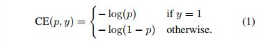
In the above y in {±1} specifies the ground-truth class and p in [0; 1] is the model’s estimated probability for the class with label y = 1. For notational convenience, we define pt:        y是真实的类别，P是模型的预测类别概率。

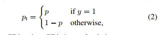
and rewrite CE(p; y) = CE(pt) = - log(pt).  由于pt比p做了变换，可以直接变为这个式子。

The CE loss can be seen as the blue (top) curve in Figure 1. One notable property of this loss, which can be easily seen in its plot, is that even examples that are easily classified (pt  :5) incur a loss with non-trivial magnitude. When summed over a large number of easy examples, these small loss values can overwhelm the rare class.

在图1中，CE损耗可以看作是蓝色（顶部）曲线。这种损失的一个显著特点是，即使是易于分类的例子（pt:5）也会产生较大的损失，这一点在图中很容易看出。当通过大量简单的例子进行总结时，这些小的损失值可以压倒少数的类。

3.1 Balanced Cross Entropy

A common method for addressing class imbalance is to introduce a weighting factor α 2 [0; 1] for class 1 and 1-α for class -1. In practice α may be set by inverse class frequency or treated as a hyperparameter to set by cross validation. For notational convenience, we define αt analogously to how we defined pt. We write the α-balanced CE loss as: 解决类不平衡的一种常用方法是为类1引入加权因子α2属于[0；1]，为类-1引入加权因子α1。实际上，α可以通过类频率的倒数来设置，也可以作为超参数通过交叉验证来设置。为了便于注释，我们将αt的定义类似于我们对pt的定义。我们将α-平衡交叉熵损失写成：

This loss is a simple extension to CE that we consider as an experimental baseline for our proposed focal loss.

这个损失是对交叉熵损失的一个简单扩展，我们认为它是我们提出的focal loss的实验基线。

3.2 Focal Loss Definition

As our experiments will show, the large class imbalance encountered during training of dense detectors overwhelms the cross entropy loss. Easily classified negatives comprise the majority of the loss and dominate the gradient. While α balances the importance of positive/negative examples, it does not differentiate between easy/hard examples. Instead, we propose to reshape the loss function to down-weight easy examples and thus focus training on hard negatives. More formally, we propose to add a modulating factor (1 - pt)γ to the cross entropy loss, with tunable focusing parameter γ ≥ 0. We define the focal loss as:

正如我们的实验所显示的，在训练稠密检测器时遇到的大类不平衡压倒了交叉熵损失。容易分类的负类占了损失的大部分，并且控制了梯度。虽然α平衡了正/负例子的重要性，但它不区分简单/困难的例子。相反，我们建议重塑减肥功能，以减轻体重，简单的例子，因此重点训练硬消极。在形式上，我们建议在交叉熵损失中加入调制因子（1-pt）γ，可调聚焦参数γ≥0。我们将焦点损失定义为：

The focal loss is visualized for several values of γ in [0; 5] in Figure 1. We note two properties of the focal loss. (1) When an example is misclassified and pt is small, the modulating factor is near 1 and the loss is unaffected. As pt -> 1, the factor goes to 0 and the loss for well-classified examples is down-weighted. (2) The focusing parameter γ smoothly adjusts the rate at which easy examples are downweighted. When γ = 0, FL is equivalent to CE, and as γ is increased the effect of the modulating factor is likewise increased (we found γ = 2 to work best in our experiments).

focal loss在图1中显示了结果，其中参数γ 在0到5 之间变化。可以看出focal loss具有两个特性：（1）当样本被错分并且pt很小时，修正项接近1，损失几乎不变。随着pt趋向于1，修正参数取向于0，也就是正确分类的样本的权重被降低了。（2）参数γ 对正确分类的简单样本的适应是平滑变化的。当γ 为0时，FL=CE,当γ 增大时，条件的效果增强了。（在我们的实验中设置了γ 为2）

Intuitively, the modulating factor reduces the loss contribution from easy examples and extends the range in which an example receives low loss. For instance, with γ = 2, an example classified with pt = 0:9 would have 100× lower loss compared with CE and with pt ≈ 0:968 it would have 1000× lower loss. This in turn increases the importance of correcting misclassified examples (whose loss is scaled down by at most 4× for pt ≤ :5 and γ = 2).

直观地，调制因子减少了简单示例的损失贡献，并且扩展了示例接收低损耗的范围。例如，当γ=2时，当pt=0:9时，与CE相比，损耗降低100倍；当pt≈0:968时，损耗降低1000倍。这又增加了纠正错误分类示例的重要性（对于pt≤：5和γ=2，其损失最多缩小4倍）。

In practice we use an α-balanced variant of the focal loss:  实际上，我们使用focal loss的α-平衡变量：

We adopt this form in our experiments as it yields slightly improved accuracy over the non-α-balanced form. Finally, we note that the implementation of the loss layer combines the sigmoid operation for computing p with the loss computation, resulting in greater numerical stability.

我们在实验中采用了这种形式，因为它比非α-平衡形式的精度稍有提高。最后，我们注意到损失层的实现将计算p的sigmoid运算与损失计算结合起来，从而产生更大的数值稳定性。

While in our main experimental results we use the focal loss definition above, its precise form is not crucial. In the appendix we consider other instantiations of the focal loss and demonstrate that these can be equally effective.

虽然在我们的主要实验结果中，我们使用了上述的focal loss定义，但它的精确形式并不重要。在附录中，我们考虑了focal loss的其他实例，并证明了这些实例同样有效。

3.3 Class Imbalance and Model Initialization

 

 

Binary classification models are by default initialized to have equal probability of outputting either y = -1 or 1. Under such an initialization, in the presence of class imbalance, the loss due to the frequent class can dominate total loss and cause instability in early training. To counter this, we introduce the concept of a ‘prior’ for the value of p estimated by the model for the rare class (foreground) at the start of training. We denote the prior by π and set it so that the model’s estimated p for examples of the rare class is low, e.g. 0.01. We note that this is a change in model initialization (see x4.1) and not of the loss function. We found this to improve training stability for both the cross entropy and focal loss in the case of heavy class imbalance.

默认情况下，二进制分类模型初始化为输出y=-1或1的概率相等。在这样的初始化条件下，在存在类别不平衡的情况下，出现多的类别损失会主导全员损失，造成早期训练的不稳定。为了解决这一问题，我们引入了“先验”的概念，用于训练开始时稀有类（前景）模型估计的p值。我们用π来表示先验，并设置它，使得对于稀有类的例子，模型的估计p是低的，例如0.01。我们注意到这是模型初始化（见x4.1）的变化，而不是损失函数的变化。我们发现在重类不平衡的情况下，这可以提高交叉熵和focal loss的训练稳定性。

3.4 Class Imbalance and Two-stage Detectors

Two-stage detectors are often trained with the cross entropy loss without use of α-balancing or our proposed loss. Instead, they address class imbalance through two mechanisms: (1) a two-stage cascade and (2) biased minibatch sampling. The first cascade stage is an object proposal mechanism [35, 24, 28] that reduces the nearly infinite set of possible object locations down to one or two thousand. Importantly, the selected proposals are not random, but are likely to correspond to true object locations, which removes the vast majority of easy negatives. When training the second stage, biased sampling is typically used to construct minibatches that contain, for instance, a 1:3 ratio of positive to negative examples. This ratio is like an implicit α- balancing factor that is implemented via sampling. Our proposed focal loss is designed to address these mechanisms in a one-stage detection system directly via the loss function.

在不使用α-平衡或我们提出的损失的情况下，两级检测器通常使用交叉熵损失进行训练。相反，它们通过两种机制解决类不平衡问题：（1）两级级联和（2）有偏小批量采样。第一个级联阶段是一个对象建议机制[35，24，28]，它将几乎无限的一组可能的对象位置减少到1千或2千个。重要的是，所选方案不是随机的，而是可能与真实的目标位置相对应，从而消除了绝大多数容易产生的负面影响。在训练第二阶段时，通常使用有偏采样来构造小批量，其中包含1:3的正负示例比率。这个比率就像是一个隐含的α-平衡因子，通过采样实现。我们提出的focal loss是为了直接通过损失函数解决单级检测系统中的这些机制。

4. RetinaNet Detector

RetinaNet is a single, unified network composed of a backbone network and two task-specific subnetworks. The backbone is responsible for computing a convolutional feature map over an entire input image and is an off-the-self convolutional network. The first subnet performs convolutional object classification on the backbone’s output; the second subnet performs convolutional bounding box regression. The two subnetworks feature a simple design that we propose specifically for one-stage, dense detection, see Figure 3. While there are many possible choices for the details of these components, most design parameters are not particularly sensitive to exact values as shown in the experiments. We describe each component of RetinaNet next.

RetinaNet是一个单一的、统一的网络，由一个骨干网和两个特定于任务的子网组成。主干网负责计算整个输入图像上的卷积特征映射，并且是一个非自卷积网络。第一个子网对骨干网的输出进行卷积对象分类；第二个子网进行卷积包围盒回归。这两个子网是我们专门为一级密集检测提出的，见图3。虽然对于这些部件的细节有许多可能的选择，但大多数设计参数对实验中所示的精确值并不特别敏感。接下来我们描述RetinaNet的每个组成部分。

Feature Pyramid Network Backbone: We adopt the Feature Pyramid Network (FPN) from [20] as the backbone network for RetinaNet. In brief, FPN augments a standard convolutional network with a top-down pathway and lateral connections so the network efficiently constructs a rich, multi-scale feature pyramid from a single resolution input image, see Figure 3(a)-(b). Each level of the pyramid can be used for detecting objects at a different scale. FPN improves multi-scale predictions from fully convolutional networks (FCN) [23], as shown by its gains for RPN [28] and DeepMask-style proposals [24], as well at two-stage detectors such as Fast R-CNN [10] or Mask R-CNN [14]. Following [20], we build FPN on top of the ResNet architecture [16]. We construct a pyramid with levels P3 through P7, where l indicates pyramid level (Pl has resolution 2l lower than the input). As in [20] all pyramid levels have C = 256 channels. Details of the pyramid generally follow [20] with a few modest differences.2 While many design choices are not crucial, we emphasize the use of the FPN backbone is; preliminary experiments using features from only the final ResNet layer yielded low AP.

采用文献[20]中的特征金字塔网络（FPN）作为RetinaNet的骨干网。简言之，FPN通过自上而下的路径和横向连接来增强标准卷积网络，因此该网络有效地从单分辨率输入图像构建丰富的多尺度特征金字塔，见图3（a）-（b）。金字塔的每一层都可以用来检测不同尺度的物体。FPN改进了来自完全卷积网络（FCN）的多尺度预测[23]，这一点在RPN[28]和DeepMask风格的建议[24]以及两级检测器（如Fast R-CNN[10]或Mask R-CNN[14]）中得到了证明。根据[20]，我们在ResNet架构的基础上构建FPN[16]。我们构造了一个P3到P7层的金字塔，其中l表示金字塔层（Pl的分辨率比输入低2l）。如[20]所示，所有金字塔级别都有C=256个通道。金字塔的细节一般遵循[20]并有一些适度的差异。2虽然许多设计选择并不重要，但我们强调使用FPN主干网是；初步实验仅使用来自最终ResNet层的特性产生低AP。

Anchors: We use translation-invariant anchor boxes similar to those in the RPN variant in [20]. The anchors have areas of 322 to 5122 on pyramid levels P3 to P7, respectively. As in [20], at each pyramid level we use anchors at three aspect ratios [1:2; 1:1, 2:1]. For denser scale coverage than in [20], at each level we add anchors of sizes [2^0，2^1/3，2^2/3] of the original set of 3 aspect ratio anchors. This improve AP in our setting. In total there are A = 9 anchors per level and across levels they cover the scale range 32 - 813 pixels with respect to the network’s input image.

我们使用类似于[20]中RPN变体的平移不变锚定框。锚的面积为322至5122，分别位于金字塔的P3至P7层。如[20]，在每个金字塔级别上，我们使用三个长宽比为[1:2；1:1，2:1]的锚。对于比[20]更密集的比例覆盖，在每个级别上，我们添加尺寸为[2^0，2^1/3，2^2/3]的原3个长宽比锚。这改善了我们的环境。总的来说，每层有9个锚定，并且跨层锚定覆盖网络输入图像的32-813像素范围。

Each anchor is assigned a length K one-hot vector of classification targets, where K is the number of object classes, and a 4-vector of box regression targets. We use the assignment rule from RPN [28] but modified for multiclass detection and with adjusted thresholds. Specifically, anchors are assigned to ground-truth object boxes using an intersection-over-union (IoU) threshold of 0.5; and to background if their IoU is in [0, 0.4). As each anchor is assigned to at most one object box, we set the corresponding entry in its length K label vector to 1 and all other entries to 0. If an anchor is unassigned, which may happen with overlap in [0.4, 0.5), it is ignored during training. Box regression targets are computed as the offset between each anchor and its assigned object box, or omitted if there is no assignment.

每个锚都被赋予一个长度K的one-hot分类目标，其中K是对象类的数量，以及一个4维矢量作为回归目标。我们使用RPN[28]中的赋值规则，但对多类检测和调整阈值进行了修改。具体地说，使用超过并集（IoU）阈值0.5的交集将锚分配给地面真值对象框；如果它们的IoU在[0，0.4]中，则将锚分配给背景。当每个锚被分配给最多一个对象框时，我们将其长度K标签向量中的相应条目设置为1，将所有其他条目设置为0。如果锚是未分配的，则可能在[0.4，0.5]中发生重叠。

Classification Subnet: The classification subnet predicts the probability of object presence at each spatial position for each of the A anchors and K object classes. This subnet is a small FCN attached to each FPN level; parameters of this subnet are shared across all pyramid levels. Its design is simple. Taking an input feature map with C channels from a given pyramid level, the subnet applies four 3×3 conv layers, each with C filters and each followed by ReLU activations, followed by a 3×3 conv layer with KA filters. Finally sigmoid activations are attached to output the KA binary predictions per spatial location, see Figure 3 (c). We use C = 256 and A = 9 in most experiments.

In contrast to RPN [28], our object classification subnet is deeper, uses only 3×3 convs, and does not share parameters with the box regression subnet (described next). We found these higher-level design decisions to be more important than specific values of hyperparameters.

分类子网：分类子网预测A个锚和K个目标类在每个空间位置的存在概率。此子网是附加到每个FPN级别的小型FCN；此子网的参数在所有金字塔级别上共享。它的设计很简单。子网从给定的金字塔级别获取一个带有C通道的输入特征映射，然后应用四个3×3 conv层，每个层都有C个过滤器，每个层都有ReLU激活，然后是一个带KA过滤器的3×3 conv层。最后，sigmoid激活被附加到每个空间位置输出KA二进制预测，参见图3（c）。我们在大多数实验中使用C=256和A=9。

与RPN[28]相比，我们的对象分类子网更深，仅使用3×3 conv，并且不与box回归子网共享参数（下面将介绍）。我们发现这些更高层次的设计决策比超参数的特定值更重要。

Box Regression Subnet: In parallel with the object classification subnet, we attach another small FCN to each pyramid level for the purpose of regressing the offset from each anchor box to a nearby ground-truth object, if one exists. The design of the box regression subnet is identical to the classification subnet except that it terminates in 4A linear outputs per spatial location, see Figure 3 (d). For each of the A anchors per spatial location, these 4 outputs predict the relative offset between the anchor and the groundtruth box (we use the standard box parameterization from RCNN [11]). We note that unlike most recent work, we use a class-agnostic bounding box regressor which uses fewer parameters and we found to be equally effective. The object classification subnet and the box regression subnet, though sharing a common structure, use separate parameters.

回归子网：与对象分类子网并行，我们在每个金字塔层附加另一个小FCN，以便将每个锚定盒的偏移量回归到附近的真值（如果存在）。回归子网的设计与分类子网相同，只是它在每个空间位置输出4A个线性结果，见图3（d）。对于每个空间位置的A个锚，这4个预测锚和真实框之间的相对偏移（我们使用RCNN[11]中的标准框参数化）。我们注意到，与最近的工作不同，我们使用一个类不可知的边界盒回归器，它使用较少的参数，但同样有效。对象分类子网和框回归子网虽然共享一个公共结构，但使用单独的参数。

4.1 Inference and Training

Inference: RetinaNet forms a single FCN comprised of a ResNet-FPN backbone, a classification subnet, and a box regression subnet, see Figure 3. As such, inference involves simply forwarding an image through the network. To improve speed, we only decode box predictions from at most 1k top-scoring predictions per FPN level, after thresholding detector confidence at 0.05. The top predictions from all levels are merged and non-maximum suppression with a threshold of 0.5 is applied to yield the final detections.

RetinaNet形成一个由ResNet FPN主干网、分类子网和box回归子网组成的FCN，见图3。为了提高速度，在阈值检测器置信度为0.05后，我们仅从每个FPN级别最多解码预测1k个最高得分。合并所有级别的顶级预测，并应用阈值为0.5的非最大抑制来产生最终检测结果。

Focal Loss: We use the focal loss introduced in this work as the loss on the output of the classification subnet. As we will show in x5, we find that γ = 2 works well in practice and the RetinaNet is relatively robust to γ 2 [0:5; 5]. We emphasize that when training RetinaNet, the focal loss is applied to all ∼100k anchors in each sampled image. This stands in contrast to common practice of using heuristic sampling (RPN) or hard example mining (OHEM, SSD) to select a small set of anchors (e.g., 256) for each minibatch. The total focal loss of an image is computed as the sum of the focal loss over all ∼100k anchors, normalized by the number of anchors assigned to a ground-truth box. We perform the normalization by the number of assigned anchors, not total anchors, since the vast majority of anchors are easy negatives and receive negligible loss values under the focal loss. Finally, we note that α, the weight assigned to the rare class, also has a stable range, but it interacts with γ making it necessary to select the two together (see Tables 1a and 1b). In general, α should be decreased slightly as γ is increased (for γ = 2, α = 0:25 works best).

Focal Loss: 我们使用在这项工作中引入的焦点损失作为分类子网输出上的损失。正如我们在x5中所展示的，我们发现γ=2在实际中工作良好，并且RetinaNet对γ2相对稳定[0:5；5]。我们强调在训练RetinaNet时，每个采样图像中的所有100k个锚都会受到焦距损失的影响。这与使用启发式采样（RPN）或硬示例挖掘（OHEM，SSD）为每个小批量选择一组锚（例如256）的常见做法形成了对比。图像的总焦距损失被计算为所有∼100k个锚的焦距损失之和，通过指定给地面真值框的锚的数量进行归一化。由于绝大多数锚都是易负的，并且在焦点损失下得到的损失值可以忽略不计，所以我们通过指定锚的数量而不是总锚的数量来执行标准化。最后，我们注意到，分配给稀有类的权重α也有一个稳定的范围，但它与γ相互作用，因此有必要同时选择两者（见表1a和1b）。一般来说，随着γ的增加，α应略微降低（对于γ=2，α=0:25效果最好）。

Initialization: We experiment with ResNet-50-FPN and ResNet-101-FPN backbones [20]. The base ResNet-50 and ResNet-101 models are pre-trained on ImageNet1k; we use the models released by [16]. New layers added for FPN are initialized as in [20]. All new conv layers except the final one in the RetinaNet subnets are initialized with bias b = 0 and a Gaussian weight fill with σ = 0:01. For the final conv layer of the classification subnet, we set the bias initialization to b = - log((1 - π)=π), where π specifies that at the start of training every anchor should be labeled as foreground with confidence of ∼π. We use π = :01 in all experiments, although results are robust to the exact value. As explained in x3.3, this initialization prevents the large number of background anchors from generating a large, destabilizing loss value in the first iteration of training.

初始化：我们使用ResNet-50-FPN和ResNet-101-FPN主干进行实验[20]。基本的ResNet-50和ResNet-101模型是在ImageNet1k上预先训练的；我们使用[16]发布的模型。为FPN添加的新层初始化为[20]。除RetinaNet子网中的最后一层外，所有新的conv层都用偏置b=0和高斯权重填充σ=0.01进行初始化。对于分类子网的最后一个conv层，我们将偏差初始化设置为b=-log（（1-π）=π），其中π指定在训练开始时，每个锚都应标记为前景，置信度为∼π。我们在所有实验中都使用π=：01，尽管结果对精确值是稳健的。如x3.3所述，该初始化防止大量背景锚在训练的第一次迭代中产生大的、不稳定的损失值。

Optimization: RetinaNet is trained with stochastic gradient descent (SGD). We use synchronized SGD over 8 GPUs with a total of 16 images per minibatch (2 images per GPU). Unless otherwise specified, all models are trained for 90k iterations with an initial learning rate of 0.01, which is then divided by 10 at 60k and again at 80k iterations. We use horizontal image flipping as the only form of data augmentation unless otherwise noted. Weight decay of 0.0001 and momentum of 0.9 are used. The training loss is the sum the focal loss and the standard smooth L1 loss used for box regression [10]. Training time ranges between 10 and 35 hours for the models in Table 1e.

优化：用随机梯度下降（SGD）训练RetinaNet 。我们使用同步SGD超过8个GPU，每个小批量总共16个图像（每个GPU 2个图像）。除非另有说明，否则所有模型都经过90k次迭代的训练，初始学习率为0.01，然后在60k次迭代时除以10，在80k次迭代时再次除以10。我们使用水平图像翻转作为数据增强的唯一形式，除非另有说明。重量衰减为0.0001，动量为0.9。训练损失是focal loss和smooth L1 loss的总和。

5. Experiments

We present experimental results on the bounding box detection track of the challenging COCO benchmark [21]. For training, we follow common practice [1, 20] and use the COCO trainval35k split (union of 80k images from train and a random 35k subset of images from the 40k image val split). We report lesion and sensitivity studies by evaluating on the minival split (the remaining 5k images from val). For our main results, we report COCO AP on the test-dev split, which has no public labels and requires use of the evaluation server.

我们给出了具有挑战性的COCO基准的预测框检测的实验结果。对于训练，我们遵循常见实践[1，20]并使用COCO train val 35k分割（将来自训练的80k图像和来自40k图像val分割的35k图像的随机子集合并）。我们报告了通过评估最小val分裂（剩余的5k val图像）的病态和敏感性研究。对于我们的主要结果，我们在test-dev split上报告COCO AP，它没有公共标签，需要使用评估服务器。

5.1 Training Dense Detection

We run numerous experiments to analyze the behavior of the loss function for dense detection along with various optimization strategies. For all experiments we use depth 50 or 101 ResNets [16] with a Feature Pyramid Network (FPN) [20] constructed on top. For all ablation studies we use an image scale of 600 pixels for training and testing.

我们进行了大量的实验来分析密度检测的损失函数的行为以及各种优化策略。对于所有的实验，我们使用深度为50或101的ResNets[16]，在上面构造一个特征金字塔网络（FPN）[20]。对于所有的研究，我们使用600像素的图像尺度进行训练和测试。

Network Initialization: Our first attempt to train RetinaNet uses standard cross entropy (CE) loss without any modifications to the initialization or learning strategy. This fails quickly, with the network diverging during training. However, simply initializing the last layer of our model such that the prior probability of detecting an object is π = :01 (see x4.1) enables effective learning. Training RetinaNet with ResNet-50 and this initialization already yields a respectable AP of 30.2 on COCO. Results are insensitive to the exact value of π so we use π = :01 for all experiments.

网络初始化：我们第一次尝试训练RetinaNet使用标准交叉熵（CE）损失，没有任何修改初始化或学习策略。这很快就失败了，网络在训练过程中出现了分化。然而，只要初始化我们模型的最后一层，使得检测对象的先验概率为π=：01（见x4.1），就可以实现有效的学习。用ResNet-50训练RetinaNet，这个初始化已经在COCO上产生了30.2的AP。结果对π的精确值不敏感，因此我们对所有实验都使用π=0.01。

Balanced Cross Entropy: Our next attempt to improve learning involved using the α-balanced CE loss described in x3.1. Results for various α are shown in Table 1a. Setting α = :75 gives a gain of 0.9 points AP.

平衡交叉熵：我们下一次尝试使用x3.1中描述的α平衡CE损失来改进学习。各种α的结果如表1a所示。设置α=：75可获得0.9点AP的增益。

Focal Loss: Results using our proposed focal loss are shown in Table 1b. The focal loss introduces one new hyperparameter, the focusing parameter γ, that controls the strength of the modulating term. When γ = 0, our loss is equivalent to the CE loss. As γ increases, the shape of the loss changes so that “easy” examples with low loss get further discounted, see Figure 1. FL shows large gains over CE as γ is increased. With γ = 2, FL yields a 2.9 AP improvement over the α-balanced CE loss.

For the experiments in Table 1b, for a fair comparison we find the best α for each γ. We observe that lower α’s are selected for higher γ’s (as easy negatives are down weighted, less emphasis needs to be placed on the positives). Overall, however, the benefit of changing γ is much larger, and indeed the best α’s ranged in just [.25,.75] (we tested α 2 [:01; :999]). We use γ = 2:0 with α = :25 for all experiments but α = :5 works nearly as well (.4 AP lower).

Analysis of the Focal Loss: To understand the focal loss better, we analyze the empirical distribution of the loss of a converged model. For this, we take our default ResNet- 101 600-pixel model trained with γ = 2 (which has 36.0 AP). We apply this model to a large number of random images and sample the predicted probability for ∼107 negative windows and ∼105 positive windows. Next, separately for positives and negatives, we compute FL for these samples, and normalize the loss such that it sums to one. Given the normalized loss, we can sort the loss from lowest to highest and plot its cumulative distribution function (CDF) for both positive and negative samples and for different settings for γ (even though model was trained with γ = 2).

Cumulative distribution functions for positive and negative samples are shown in Figure 4. If we observe the positive samples, we see that the CDF looks fairly similar for different values of γ. For example, approximately 20% of the hardest positive samples account for roughly half of the positive loss, as γ increases more of the loss gets concentrated in the top 20% of examples, but the effect is minor.

The effect of γ on negative samples is dramatically different. For γ = 0, the positive and negative CDFs are quite similar. However, as γ increases, substantially more weight becomes concentrated on the hard negative examples. In fact, with γ = 2 (our default setting), the vast majority of the loss comes from a small fraction of samples. As can be seen, FL can effectively discount the effect of easy negatives, focusing all attention on the hard negative examples.

Online Hard Example Mining (OHEM): [31] proposed to improve training of two-stage detectors by constructing minibatches using high-loss examples. Specifically, in OHEM each example is scored by its loss, non-maximum suppression (nms) is then applied, and a minibatch is constructed with the highest-loss examples. The nms threshold and batch size are tunable parameters. Like the focal loss, OHEM puts more emphasis on misclassified examples, but unlike FL, OHEM completely discards easy examples. We also implement a variant of OHEM used in SSD [22]: after applying nms to all examples, the minibatch is constructed to enforce a 1:3 ratio between positives and negatives to help ensure each minibatch has enough positives.

在线难例样本挖掘（OHEM）：[31]提出通过使用高损失示例构造小批量来改进两阶段检测器的训练。具体来说，在OHEM中，每个例子都是按其损失来评分的，然后应用非最大抑制（nms），并用损失最大的例子构造一个小批量。nms阈值和批处理大小是可调参数。像focal loss一样，OHEM更强调错误分类的例子，但不像FL，OHEM完全抛弃了简单的例子。我们还实现了SSD[22]中使用的OHEM变体：在将nms应用于所有示例之后，构建小批量以强制正样本和负样本之间的1:3比率，以帮助确保每个小批量都有足够的正样本。

We test both OHEM variants in our setting of one-stage detection which has large class imbalance. Results for the original OHEM strategy and the ‘OHEM 1:3’ strategy for selected batch sizes and nms thresholds are shown in Table 1d. These results use ResNet-101, our baseline trained with FL achieves 36.0 AP for this setting. In contrast, the best setting for OHEM (no 1:3 ratio, batch size 128, nms of .5) achieves 32.8 AP. This is a gap of 3.2 AP, showing FL is more effective than OHEM for training dense detectors. We note that we tried other parameter setting and variants for OHEM but did not achieve better results.

在我们的一级检测设置中，我们测试了两种OHEM变体，这两种检测具有较大的类不平衡性。原始OHEM策略和所选批量大小和nms阈值的“OHEM 1:3”策略的结果如表1d所示。这些结果使用ResNet-101，我们使用FL训练的基线在此设置下达到36.0 AP。相比之下，OHEM的最佳设置（1:3比率，批量大小128，nms为.5）达到32.8AP。这是一个3.2ap的差距，表明FL比OHEM训练密集型探测器更有效。我们注意到，我们尝试了OHEM的其他参数设置和变体，但没有取得更好的效果。

Hinge Loss: Finally, in early experiments, we attempted to train with the hinge loss [13] on pt, which sets loss to 0 above a certain value of pt. However, this was unstable and we did not manage to obtain meaningful results. Results exploring alternate loss functions are in the appendix.

5.2 Model Architecture Design

Anchor Density: One of the most important design factors in a one-stage detection system is how densely it covers the space of possible image boxes. Two-stage detectors can classify boxes at any position, scale, and aspect ratio using a region pooling operation [10]. In contrast, as one-stage detectors use a fixed sampling grid, a popular approach for achieving high coverage of boxes in these approaches is to use multiple ‘anchors’ [28] at each spatial position to cover boxes of various scales and aspect ratios.

锚密度：在一级检测系统中，最重要的设计因素之一是覆盖可能的图像框的空间有多密。两级检测器可以使用区域池操作对任何位置、比例和纵横比的框进行分类[10]。相比之下，由于一级检测器使用固定采样网格，在这些方法中，实现框的高覆盖率的流行方法是在每个空间位置使用多个“锚”[28]来覆盖不同比例和纵横比的框。

We sweep over the number of scale and aspect ratio anchors used at each spatial position and each pyramid level in FPN. We consider cases from a single square anchor at each location to 12 anchors per location spanning 4 sub-octave scales (2k=4, for k ≤ 3) and 3 aspect ratios [0.5, 1, 2]. Results using ResNet-50 are shown in Table 1c. A surprisingly good AP (30.3) is achieved using just one square anchor. However, the AP can be improved by nearly 4 points (to 34.0) when using 3 scales and 3 aspect ratios per location. We used this setting for all other experiments in this work.

我们扫描了在FPN中每个空间位置和每个金字塔级别使用的比例和纵横比锚的数量。我们考虑从每个位置的单个方形锚定到每个位置的12个锚定，跨越4个倍频标度（2k=4，对于k≤3）和3个纵横比[0.5，1，2]。使用ResNet-50的结果如表1c所示。仅使用一个方形锚定即可获得令人惊讶的良好AP（30.3）。然而，当每个位置使用3个尺度和3个纵横比时，AP可以提高近4个点（达到34.0）。在这项工作中，我们将此设置用于所有其他实验。

Finally, we note that increasing beyond 6-9 anchors did not shown further gains. Thus while two-stage systems can classify arbitrary boxes in an image, the saturation of performance w.r.t. density implies the higher potential density of two-stage systems may not offer an advantage.

最后，我们注意到，超过6-9锚没有显示出进一步的收益。因此，虽然两级系统可以对图像中的任意盒子进行分类，但性能w.r.t.密度的饱和意味着两级系统的较高密度可能不会提供优势。

Speed versus Accuracy: Larger backbone networks yield higher accuracy, but also slower inference speeds. Likewise for input image scale (defined by the shorter image side). We show the impact of these two factors in Table 1e. In Figure 2 we plot the speed/accuracy trade-off curve for RetinaNet and compare it to recent methods using public numbers on COCO test-dev. The plot reveals that RetinaNet, enabled by our focal loss, forms an upper envelope over all existing methods, discounting the low-accuracy regime. RetinaNet with ResNet-101-FPN and a 600 pixel image scale (which we denote by RetinaNet-101-600 for simplicity) matches the accuracy of the recently published ResNet- 101-FPN Faster R-CNN [20], while running in 122 ms per image compared to 172 ms (both measured on an Nvidia M40 GPU). Using larger scales allows RetinaNet to surpass the accuracy of all two-stage approaches, while still being faster. For faster runtimes, there is only one operating point (500 pixel input) at which using ResNet-50-FPN improves over ResNet-101-FPN. Addressing the high frame rate regime will likely require special network design, as in [27], and is beyond the scope of this work. We note that after publication, faster and more accurate results can now be obtained by a variant of Faster R-CNN from [12].

速度vs准确度：较大的主干网产生更高的准确度，但速度慢。同样输入图像比例也是如此（由图像的较短侧定义）。我们在表1e中显示了这两个因素的影响。在图2中，我们绘制了RetinaNet的速度/精度权衡曲线，并将其与最近在COCO test-dev中使用公共数字的方法进行了比较。该图显示，RetinaNet由于我们的focal loss，在所有现有方法上形成了一个上包络线，从而降低了低精度范围。ResNet-101-FPN的RetinaNet和600像素的图像比例（为了简单起见，我们用RetinaNet-101-600表示）与最近发布的ResNet-101-FPN的精度相匹配，R-CNN的速度更快[20]，同时每张图像的运行时间为122 ms，而不是172 ms（都是在Nvidia M40 GPU上测量的）。使用更大的比例尺可以使RetinaNet超过所有两阶段方法的准确性，同时仍然更快。对于更快的运行时间，只有一个操作点（500像素输入）使用ResNet-50-FPN比ResNet-101-FPN提高。解决高帧速率体制可能需要特殊的网络设计，如[27]所示，并且超出了本工作的范围。我们注意到，在发表后，更快更准确的结果现在可以通过快速R-CNN的变体从[12]中获得。

5.3 Comparison to State of the Art

We evaluate RetinaNet on the challenging COCO dataset and compare test-dev results to recent state-of-the-art methods including both one-stage and two-stage models. Results are presented in Table 2 for our RetinaNet-101-800 model trained using scale jitter and for 1.5× longer than the models in Table 1e (giving a 1.3 AP gain). Compared to existing one-stage methods, our approach achieves a healthy 5.9 point AP gap (39.1 vs. 33.2) with the closest competitor, DSSD [9], while also being faster, see Figure 2. Compared to recent two-stage methods, RetinaNet achieves a 2.3 point gap above the top-performing Faster R-CNN model based on Inception-ResNet-v2-TDM [32]. Plugging in ResNeXt- 32x8d-101-FPN [38] as the RetinaNet backbone further improves results another 1.7 AP, surpassing 40 AP on COCO.

我们在具有挑战性的COCO数据集上评估RetinaNet，并将测试开发结果与包括一阶段和两阶段模型的最新方法进行比较。表2显示了我们的RetinaNet-101-800模型使用比例抖动训练的结果，比表1e中的模型长1.5倍（给出1.3ap增益）。与现有的单阶段方法相比，我们的方法与最接近的竞争对手DSSD[9]的AP差距达到了5.9个点（39.1对33.2），同时速度也更快，见图2。与最近的两阶段方法相比，RetinaNet比基于Inception-ResNet-v2-TDM的性能最好的R-CNN模型高出2.3个点[32]。插入ResNeXt-32x8d-101-FPN[38]作为视网膜骨干进一步改善结果，另一个1.7ap，超过了COCO上的40ap。

6. Conclusion

In this work, we identify class imbalance as the primary obstacle preventing one-stage object detectors from surpassing top-performing, two-stage methods. To address this, we propose the focal loss which applies a modulating term to the cross-entropy loss in order to focus learning on hard negative examples. Our approach is simple and highly effective. We demonstrate its efficacy by designing a fully convolutional one-stage detector and report extensive experimental analysis showing that it achieves state-of-the-art accuracy and speed. Source code is available at https://github.com/facebookresearch/Detectron [12].

在这项工作中，我们确定类不平衡是阻止一级目标检测器超越最佳性能的两级方法的主要障碍。为了解决这一问题，我们提出了将调制项应用于交叉熵损失的焦点损失，以便将学习集中在硬的反面例子上。我们的方法简单高效。我们通过设计一个完全卷积的单级检测器来证明它的有效性，并报告了大量的实验分析，表明它达到了最先进的精度和速度。源代码可在https://github.com/facebook research/Detectron[12]上找到。

Appendix A: Focal Loss*

The exact form of the focal loss is not crucial. We now show an alternate instantiation of the focal loss that has similar properties and yields comparable results. The following also gives more insights into properties of the focal loss. We begin by considering both cross entropy (CE) and the focal loss (FL) in a slightly different form than in the main text. Specifically, we define a quantity xt as follows:

where y in {±1} specifies the ground-truth class as before. We can then write pt = σ(xt) (this is compatible with the definition of pt in Equation 2). An example is correctly classified when xt > 0, in which case pt > :5. We can now define an alternate form of the focal loss in terms of xt. We define p∗ t and FL∗ as follows:

FL∗ has two parameters, γ and β, that control the steepness and shift of the loss curve. We plot FL∗ for two selected settings of γ and β in Figure 5 alongside CE and FL. As can be seen, like FL, FL∗ with the selected parameters diminishes the loss assigned to well-classified examples. We trained RetinaNet-50-600 using identical settings as before but we swap out FL for FL∗ with the selected parameters. These models achieve nearly the same AP as those trained with FL, see Table 3. In other words, FL∗ is a reasonable alternative for the FL that works well in practice.

We found that various γ and β settings gave good results. In Figure 7 we show results for RetinaNet-50-600 with FL∗ for a wide set of parameters. The loss plots are color coded such that effective settings (models converged and with AP over 33.5) are shown in blue. We used α = :25 in all experiments for simplicity. As can be seen, losses that reduce weights of well-classified examples (xt > 0) are effective. More generally, we expect any loss function with similar properties as FL or FL∗ to be equally effective.

Appendix B: Derivatives

For reference, derivates for CE, FL, and FL*  w.r.t. x are:

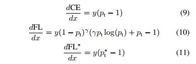
Plots for selected settings are shown in Figure 6. For all loss functions, the derivative tends to -1 or 0 for high-confidence predictions. However, unlike CE, for effective settings of both FL and FL∗, the derivative is small as soon as xt > 0.

 

总结

1.主要思想

本文指出，目前目标检测有两种类型框架：

一种是两阶段的，例如RCNN、fastRCNN、fasterRCNN、maskRCNN等这一系列的。其分为两个阶段，第一个阶段使用CNN提取到特征图之后，使用region proposal network得到类别的感兴趣区域，第二个阶段使用classifier进行类别的回归，最终实现检测，这种方式分两个步骤，检测速度比较慢，但是效果准确率很高。

另一种就是一阶段的，例如YOLO、SSN等。其直接使用CNN提到多尺度特征图之后，根据人为选定的anchor，使用不同scale和不同aspect ratios在不同尺度的feature map上进行感兴趣区域的提取，以来覆盖整个图片，然后直接对这些感兴趣anchor使用CNN进行位置和类别的回归，最后使用Non-Maximum Suppression得到最终的检测结果，一步达到检测的结果， 这种方式一步到位，检测速度较快，但是准确率相较于two-stage的方法有所下降。

这篇文章分析one-stage对于two-stage的方法准确率下降的原因在于类别分布不均不平衡，two-stage使用proposal的方法（Selective Search , EdgeBoxes ,DeepMask , RPN ）在每张图上能得到1-2k左右的感兴趣区域，很大程度上过滤掉了背景，只留下需要分类的前景，但是one-stage使用多尺度anchor的方法在每张图上能到100k左右的感兴趣区域，相当于是对全图的均匀采样，并没有区分掉背景和需要分类的前景，背景和需要分类的前景之间的数量分布不存，使用传统的交叉熵loss（-logp）会导致训练效果降低，因此检测率有所下降，因此本文提出了一种能够解决这种类别不平衡的loss，称为focal loss，为了验证这个focal loss有效，提出了one-stage网络RetinaNet来验证。

2.focal loss的提出

先从交叉熵的一般形式来提出（这里是两类分类问题，作者指出多类问题的性质相同）：

将p作改写：

带入上式得到交叉熵的形式变为：

CE(p; y) = CE(pt) = - log(pt).

另外在这个形式的基础上，提出不同类别的不平衡问题，并分别设置不同的调节参数，对于正类参数是α（在0,1之间），对于负类采用1-α，并仿照上述形式表达为：

 

但实验显示，在proposal框很密集的情况下，虽然α平衡了正/负例子的权重，但它不区分简单/困难的例子。由此在交叉熵损失中加入调制因子（1-pt)^γ。我们将focal loss定义为：

从而可以自动调节难例样本的训练权重，也就是让难样本的权重增加，迫使训练器适应难例样本。在作者的实验中，他认为γ取2时效果最好。

3.focal loss与OHEM的区别

按理来说，focal loss 和OHEM不都是对难例样本的处理吗？为什么OHEM的效果要差一点呢。

按作者的话说，OHEM采用的是对所有样本的loss排序，采用非极大值抑制的方法，只提取其中loss最大的若干样本来训练，也就是完全抛弃了简单样本的作用。这可能是导致OHEM效果不好的原因。

4. RetinaNet的网络结构

RetinaNet说到底就是resNet+FPN+两个FCN子网络的合体，FPN使得网络能够结合多尺度的特征信息。在FPN上的每层feature map上使用CNN进行class和box的子网络（虽然结构相同，但是并不共享权重）。

FPN的内容可以查看下面这张图像：

这是四种不同的生成多维度特征组合的方法。

图(a)中的方法即为常规的生成一张图片的多维度特征组合的经典方法。即对某一输入图片我们通过压缩或放大从而形成不同维度的图片作为模型输入，使用同一模型对这些不同维度的图片分别处理后，最终再将这些分别得到的特征（feature maps）组合起来就得到了我们想要的可反映多维度信息的特征集。此种方法缺点在于需要对同一图片在更改维度后输入处理多次，因此对计算机的算力及内存大小都有较高要求。

图(b)中的方法则只拿单一维度的图片做为输入，然后经CNN模型处理后，拿最终一层的feature maps作为最终的特征集。显然此种方法只能得到单一维度的信息。优点是计算简单，对计算机算力及内存大小都无过高需求。此方法为大多数R-CNN系列目标检测方法所用像R-CNN/Fast-RCNN/Faster-RCNN等。因此最终这些模型对小维度的目标检测性能不是很好。

图(c)中的方法同样是拿单一维度的图片做为输入，不过最终选取用于接下来分类或检测任务时的特征组合时，此方法不只选用了最后一层的high level feature maps，同样也会选用稍靠下的反映图片low level 信息的feature maps。然后将这些不同层次（反映不同level的图片信息）的特征简单合并起来（一般为concat处理），用于最终的特征组合输出。此方法可见于SSD当中。不过SSD在选取层特征时都选用了较高层次的网络。比如在它以VGG16作为主干网络的检测模型里面所选用的最低的Convolution的层为Conv4，这样一些具有更低级别信息的层特征像Conv2/Conv3就被它给漏掉了，于是它对更小维度的目标检测效果就不大好。

图(d)中的方法同图(c)中的方法有些类似，也是拿单一维度的图片作为输入，然后它会选取所有层的特征来处理然后再联合起来做为最终的特征输出组合。（作者在论文中拿Resnet为实例时并没选用Conv1层，那是为了算力及内存上的考虑，毕竟Conv1层的size还是比较大的，所包含的特征跟直接的图片像素信息也过于接近）。另外还对这些反映不同级别图片信息的各层自上向下进行了再处理以能更好地组合从而形成较好的特征表达（详细过程会在下面章节中进一步介绍）。而此方法正是我们本文中要讲的FPN CNN特征提取方法。