论文解读--Automatic Portrait Segmentation for Image Stylization
Automatic Portrait Segmentation for Image Stylization
论文及数据下载地址:
http://xiaoyongshen.me/webpage_portrait/index.html
Github项目地址:
https://github.com/PetroWu/AutoPortraitMatting
开门见山,文章先给我们看了本文的PortraitFCN+方法的matting效果和几个应用场景

2.Related work不再赘述了,列出了一些基于CNN的分割方法,最好的精度大约是70%,尽管已经很出色但是对于人像的matting还差一些。
3. Our Motivation and Approach
为了大家理解,文章先介绍了在分割大有作为的FCN网络:FCN uses a spatial loss function and is formulated as a pixel regression problem against the ground-truth labeled mask. The objective function can be written as, ![]()
其中p是图像的像素索引。 Xθ( p)是参数θ下p位置像素的FCN回归函数。 损失函数e(…)测量回归输出和真值ℓ( p)之间的误差。 FCN通常由以下类型的层组成:
Convolution Layers 卷基层
ReLU Layers relu激活函数层
Pooling Layers pooling层(文章用的maxpooling)
Deconvolution Layers 反卷积层
Loss Layer 损失函数层
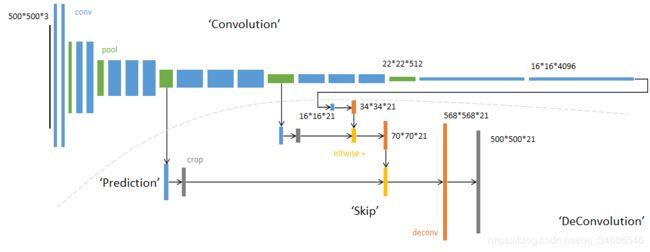
FCN: FCN对图像进行像素级的分类,从而解决了语义级别的图像分割(semantic segmentation)问题。与经典的CNN在卷积层之后使用全连接层得到固定长度的特征向量进行分类(全联接层+softmax输出)不同,FCN可以接受任意尺寸的输入图像,采用反卷积层对最后一个卷积层的feature map进行上采样, 使它恢复到输入图像相同的尺寸,从而可以对每个像素都产生了一个预测, 同时保留了原始输入图像中的空间信息, 最后在上采样的特征图上进行逐像素分类。
最后逐个像素计算softmax分类的损失, 相当于每一个像素对应一个训练样本。
在这篇博客中看到一幅很棒的图:
https://blog.csdn.net/qq_36269513/article/details/80420363
下面结合本论文开源的Github项目代码,来简单的看一下FCN在本论文中如何被应用的:
代码文件:./AutoPortraitMatting/FCN_plus.py
"""
finetune on vgg-19
"""
def vgg_net(weights, image):
    layers = (
        'conv1_1', 'relu1_1', 'conv1_2', 'relu1_2', 'pool1',

        'conv2_1', 'relu2_1', 'conv2_2', 'relu2_2', 'pool2',

        'conv3_1', 'relu3_1', 'conv3_2', 'relu3_2', 'conv3_3',
        'relu3_3', 'conv3_4', 'relu3_4', 'pool3',

        'conv4_1', 'relu4_1', 'conv4_2', 'relu4_2', 'conv4_3',
        'relu4_3', 'conv4_4', 'relu4_4', 'pool4',

        'conv5_1', 'relu5_1', 'conv5_2', 'relu5_2', 'conv5_3',
        'relu5_3', 'conv5_4', 'relu5_4'
    )

    net = {}
    current = image
    for i, name in enumerate(layers):
        if name in ['conv3_4', 'relu3_4', 'conv4_4', 'relu4_4', 'conv5_4', 'relu5_4']:
            continue
        kind = name[:4]
        if kind == 'conv':
            kernels, bias = weights[i][0][0][0][0]
            # matconvnet: weights are [width, height, in_channels, out_channels]
            # tensorflow: weights are [height, width, in_channels, out_channels]
            kernels = utils.get_variable(np.transpose(kernels, (1, 0, 2, 3)), name=name + "_w")
            bias = utils.get_variable(bias.reshape(-1), name=name + "_b")
            current = utils.conv2d_basic(current, kernels, bias)
        elif kind == 'relu':
            current = tf.nn.relu(current, name=name)
            if FLAGS.debug:
                utils.add_activation_summary(current)
        elif kind == 'pool':
            current = utils.avg_pool_2x2(current)
        net[name] = current

    return net
上面代码即vgg19的网络模型,接下来在inference函数中通过下载vgg19的预训练模型(MODEL_URL链接),对本vgg19进行初始化。并在conv5_3连接卷积层conv6,relu6和relu_dropout6,同样在relu_dropout6上连接卷积层conv7,relu7和relu_dropout7,这两层我的理解是原vgg19中的全连接层,这里用卷积层替代。conv8为114096*NUM_OF_CLASSESS(本文是2)。后续分别在conv8的输出在pooling4,和pooling3层的特征图上进行反卷积融合,得到与原图尺寸大小的结果。
def inference(image, keep_prob):
    """
    Semantic segmentation network definition
    :param image: input image. Should have values in range 0-255
    :param keep_prob:
    :return:
    """
    print("setting up vgg initialized conv layers ...")
    model_data = utils.get_model_data(FLAGS.model_dir, MODEL_URL)

    mean = model_data['normalization'][0][0][0]
    mean_pixel = np.mean(mean, axis=(0, 1))

    weights = np.squeeze(model_data['layers'])

    #processed_image = utils.process_image(image, mean_pixel)

    with tf.variable_scope("inference"):
        image_net = vgg_net(weights, image)
        conv_final_layer = image_net["conv5_3"]

        pool5 = utils.max_pool_2x2(conv_final_layer)

        W6 = utils.weight_variable([7, 7, 512, 4096], name="W6")
        b6 = utils.bias_variable([4096], name="b6")
        conv6 = utils.conv2d_basic(pool5, W6, b6)
        relu6 = tf.nn.relu(conv6, name="relu6")
        if FLAGS.debug:
            utils.add_activation_summary(relu6)
        relu_dropout6 = tf.nn.dropout(relu6, keep_prob=keep_prob)

        W7 = utils.weight_variable([1, 1, 4096, 4096], name="W7")
        b7 = utils.bias_variable([4096], name="b7")
        conv7 = utils.conv2d_basic(relu_dropout6, W7, b7)
        relu7 = tf.nn.relu(conv7, name="relu7")
        if FLAGS.debug:
            utils.add_activation_summary(relu7)
        relu_dropout7 = tf.nn.dropout(relu7, keep_prob=keep_prob)

        W8 = utils.weight_variable([1, 1, 4096, NUM_OF_CLASSESS], name="W8")
        b8 = utils.bias_variable([NUM_OF_CLASSESS], name="b8")
        conv8 = utils.conv2d_basic(relu_dropout7, W8, b8)
        # annotation_pred1 = tf.argmax(conv8, dimension=3, name="prediction1")

        # now to upscale to actual image size
        deconv_shape1 = image_net["pool4"].get_shape()
        W_t1 = utils.weight_variable([4, 4, deconv_shape1[3].value, NUM_OF_CLASSESS], name="W_t1")
        b_t1 = utils.bias_variable([deconv_shape1[3].value], name="b_t1")
        conv_t1 = utils.conv2d_transpose_strided(conv8, W_t1, b_t1, output_shape=tf.shape(image_net["pool4"]))
        fuse_1 = tf.add(conv_t1, image_net["pool4"], name="fuse_1")

        deconv_shape2 = image_net["pool3"].get_shape()
        W_t2 = utils.weight_variable([4, 4, deconv_shape2[3].value, deconv_shape1[3].value], name="W_t2")
        b_t2 = utils.bias_variable([deconv_shape2[3].value], name="b_t2")
        conv_t2 = utils.conv2d_transpose_strided(fuse_1, W_t2, b_t2, output_shape=tf.shape(image_net["pool3"]))
        fuse_2 = tf.add(conv_t2, image_net["pool3"], name="fuse_2")

        shape = tf.shape(image)
        deconv_shape3 = tf.stack([shape[0], shape[1], shape[2], NUM_OF_CLASSESS])
        W_t3 = utils.weight_variable([16, 16, NUM_OF_CLASSESS, deconv_shape2[3].value], name="W_t3")
        b_t3 = utils.bias_variable([NUM_OF_CLASSESS], name="b_t3")
        conv_t3 = utils.conv2d_transpose_strided(fuse_2, W_t3, b_t3, output_shape=deconv_shape3, stride=8)

        annotation_pred = tf.argmax(conv_t3, dimension=3, name="prediction")

    return tf.expand_dims(annotation_pred, dim=3), conv_t3
通过该FCN在作者们制作的肖像数据集中训练能够得到不错的结果,如下图(c),在服装和背景区域仍然存在问题。 其中一个重要原因就是CNN固有的平移不变性。 随后的卷积和池化层逐步交换空间信息以获取语义信息。 虽然这对分类这样的任务来说是可取的,但这意味着我们失去了允许网络学习的信息,例如,4(c)中上方和脸部右侧看上去应是背景。
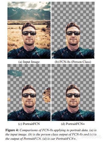
所以这才引出本文真正的大招(PortraitFCN+ model)
3.3 our Approach

FCN+的主要改进是对数据预处理,网络输入六通道的数据而不是之前的三通道。主要过程是先利用面部特征检测器(facial feature detectors )去生成辅助的位置和形状通道,这些通道与肖像的颜色信息(三通道)一起输入到网络的第一个卷积层中。
位置通道
位置通道为2通道,分别是标准化的x通道与y通道。先通过面部特征检测器检测出特征点,并估算出一个homograph单应变换矩阵τ(拟合特征和典型姿态之间的变换矩阵原文是:a homography transform T between the fitted features and a canonical pose as shown in Figure 3 (d))。将归一化的 x 通道定义为 τ(ximg) ,其中 ximg 是图像中脸部中心为零的像素的x坐标。 我们同样类似地定义标准化的 y 通道。 直观地说,该过程表示在以脸部为中心的坐标系中各个像素的位置,并根据面部尺寸进行了缩放。
形状通道
形状通道及一个单通道的meanmask图像,用来作为一个大概的人像特征(最终结果的合理估计)。那么如何得到这个合理估计呢,作者是通过计算训练集的mask均值(aligned后的及对其后的mask均值),每个训练集都有对应的肖像图和mask图(肖像-掩膜对{Pi,Mi}),通过用上面提到过的拟合面部特征点和典型姿态之间的单应变换矩阵对Mi进行变化(应该是一个aligned操作)。计算meanmask的公式如下:

其中wi是一个矩阵,指示Mi中的像素经过Ti变换后是否处于图像之外。 如果像素位于图像内,则值为1,否则设为0。 运算符◦表示元素乘法。 这意味着已经和典型姿态对齐的掩膜M接下来可以类似地变换为与输入肖像的脸部特征点对齐。
看看代码(Matlab)帮助理解,也可以跳过代码,无伤大雅
if size(tracker,1)==49
	 [tform,~,~] = estimateGeometricTransform(double(reftrack)+repmat([600 600],[49 1]),...#计算单应变换矩阵
	 double(tracker)+repmat([600 600],[49 1]),'affine');//tracker是检测的人脸图
	 outputView = imref2d(size(xxc));//xxc = (xxc-600-refpos(1))/600
	 warpedxx = imwarp(xxc,tform,'OutputView',outputView);
	 warpedyy = imwarp(yyc,tform,'OutputView',outputView);//;yyc = (yyc-600-refpos(2))/800;
	 warpedmask = imwarp(maskc,tform,'OutputView',outputView);//maskc为载入的计算好的meanmask图

	 warpedxx = warpedxx(601:1400,601:1200,:);//800,600
	 warpedyy = warpedyy(601:1400,601:1200,:);//800,600
	 warpedmask = warpedmask(601:1400,601:1200,:);//800,600

	 //PortraitFCN data
	 save(['portraitFCN_data/' imgname(1:end-4) '.mat'],'img');
	 //普通fcn只是存为3通道,作为卷积层输入
	 //下面FCN+方法组合了标准化的xx,yy和meanmask通道
	 //portraitFCN+ data
	 imgcpy = img;
	 img = zeros(800,600,6);
	 img(:,:,1:3) = imgcpy;
	 img(:,:,4) = warpedxx;
	 img(:,:,5) = warpedyy;
 	 img(:,:,6) = warpedmask;
 	 save(['portraitFCN+_data/' imgname(1:end-4) '.mat'],'img');
else
    //PortraitFCN data
    save(['portraitFCN_data/' imgname(1:end-4) '.mat'],'img');

   // portraitFCN+ data
    imgcpy = img;
    img = zeros(800,600,6);
    img(:,:,1:3) = imgcpy;
    save(['portraitFCN+_data/' imgname(1:end-4) '.mat'],'img');
这里为什么根据tracker(1)的size等于49进行判断?两个分支的区别是什么,我还不大清楚,有知道的大佬可以留言告诉我一哈
4. Data and Model Training
这一节介绍数据集。1800张portrait images 来自 Flickr并且人工用PS进行了标记,使用face detector对每张图片裁剪成600*800的size,1800分成1500张training dataset,300张testing/validation dataset(测试和交叉验证集放在一起?可能只是意思这300张用来测试吧),后续还对数据进行了图像增强,包括尺度缩放,旋转和gamma变换,生成了19000张训练图片。我们能下载到的只有未做数据增强的图片。

模型训练:

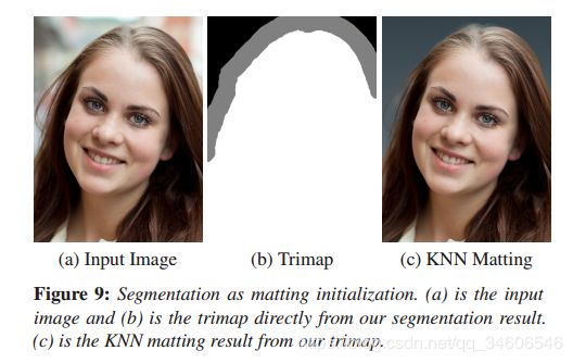
第五章是一些评估内容和展示结果还有列举出一些应用场景,读着可以在文章中细细品味,这里主要关注5.2 post processing,为什么要着重关注呢,因为这里文章提供了产生trimap的方法,而trimap是做matting必不可少的一部分。另外一个原因是我在跑TensorFlow的代码的时候,生成的trimap并不大正确,严格的说是完全错误的。可能不是caffe的代码,或者说tf的代码中在生成trimap的时候有一些逻辑上的错误?我还会继续研究,待有结果更新博客。
文章给出的trimap图:
我自己生成的分割图和trimap图:

放大这个trimap看一下(小女孩很可爱 …):
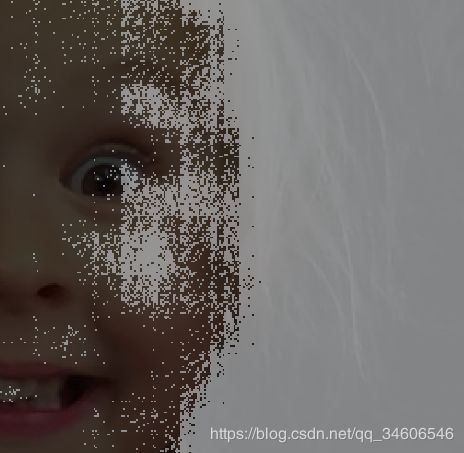
可见,这个trimap不是按照分割边界的10像素点作为Unknown这种逻辑产生的(原文:Our estimated segmentation result provides a good trimap initialization for image matting. As shown in Figure 9, we generate a trimap by setting the pixels within a 10-pixel radius of the segmentation
boundary as the “unknown”. )。
对于文章对应用场景的列举这里就不在赘述了,有兴趣可以仔细阅读下文章。最后善始善终,贴出原文的Conclusion作为总结。
- Conclusions and Future Work
In this paper we propose a high performance automatic portrait segmentation method. The system is built on deep convolutional neural network which is able to leverage portrait specific cues. We construct a large portrait image dataset with enough portrait segmentation and ground-truth data to enable effective training and testing of our model. Based on the efficient segmentation, a number of automatic portrait applications are demonstrated. Our system could fail when the background and foreground have very small contrast. We treat this as the limitation of our method. In the future, we will improve our model for higher accuracy and extend the framework to the portrait video segmentation.