WS-DAN:Weakly Supervised Data Augmentation Netowrk for Fine-Grained Visual Classification
See Better Before Looking Closer: Weakly Supervised Data Augmentation Netowrk for Fine-Grained Visual Classification
Paper PDF
文章目录
- Abstract
- Innovation
- Pipeline
- Weakly Supervised Attention Learning
- Spatial Representation
- Bilinear Attention Pooling(BAP)
- Attention Regularization
- Attention-guided Data Augmentation
- Augmentation Map
- Attention Cropping
- Attention Dropping
- Object Localization and Refinement
- Experiments
- Ablation:
- Comparison with random data augmentation
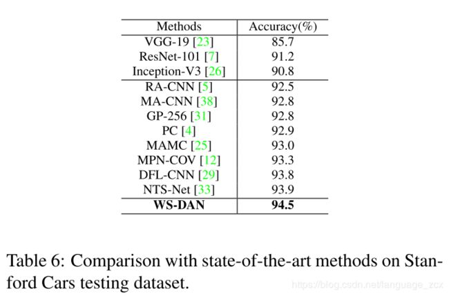
- Comparison with Stage-of-the-Art Methods
Abstract
In practice, random data augmentation, such as random image cropping, is low-efficiency and might introduce many uncontrolled background noises. In this paper, they propose Weakly Supervised Data Augmentation Network (WS-DAN) to explore the potential of data augmentation. Specifically, for each training image, we first generate attention maps to represent the object’s discriminative parts by weakly supervised learning. Next, we augment the image guided by these attention maps, including attention cropping and attention dropping. The proposed WS-DAN improves the classification accuracy in two folds. In the first stage, images can be seen better since more discriminative parts’ features will be extracted. In the second stage, attention regions provide accurate location of object, which ensures our model to look at the object closer and further improve the performance.
In summary, the main contributions of this work are:
- They propose Weakly Supervised Attention Learning to generate attention maps to represent the spatial distribution of discriminative object’s parts, And use BAP module to get the whole object feature by accumulating the object’s part feature.
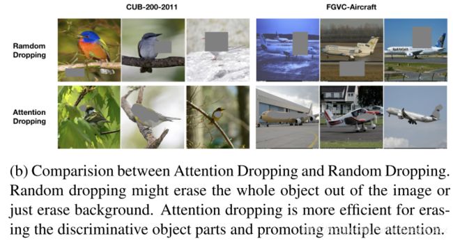
- Based on attention maps, they propose attention-guided data augmentation to improve the efficiency of data augmentation, including attention cropping and attention dropping. Attention cropping randomly crops and resizes one of the attention part to enhance the local feature representation. Attention dropping randomly erases one of the attention region out of the image in order to encourage the model to extract the feature from multiple discriminative parts.
- They utilize attention maps to accurately locate the whole object and enlarge it to further improve the classification accuracy.
Innovation
- Bilinear Attention Pooling(BAP)
- Attention Regularization
- Attention-guided Data Augmentation
Pipeline

The training process can be divided into two parts: Weakly Supervised Attention Learning and Attention-guided Data Augmentation:
Weakly Supervised Attention Learning
Spatial Representation
Attention maps A which is obtained from Feature maps F by convolutional function f ( ⋅ ) f(\cdot) f(⋅) in Equ 1 . Each Attention map A k A_{k} Ak represents one of the object’s part or visual pattern, such as the head of a bird, the wheel of a car or the wing of an aircraft. Attention maps will be utilized to augment training data.
A = f ( F ) = ⋃ k = 1 M A k (1) A=f(F)=\bigcup_{k=1}^{M}A_{k} \tag{1} A=f(F)=k=1⋃MAk(1)
Bilinear Attention Pooling(BAP)
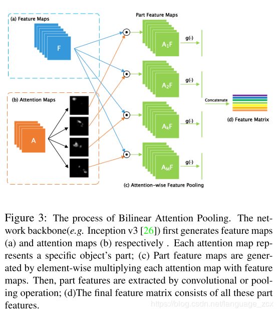
They propose Bilinear Attention Pooling (BAP) to extract features from these parts are represented by Attention maps. We element-wise multiply feature maps F by each attention map A k A_{k} Ak in order to generate M part feature maps F k F_{k} Fk, as shown in Equ 2
F k = A k ⊙ F ( k = 1 , 2 , . . . , M ) (2) F_{k} = A_{k} \odot F (k = 1, 2, ...,M) \tag{2} Fk=Ak⊙F(k=1,2,...,M)(2)
Then, They further extract discriminative local feature by additional feature extraction function g ( ⋅ ) g(\cdot) g(⋅) such as Global Average Pooling (GAP), Global Maximum Pooling (GMP) or convolutions, in order to obtain k t h k_{th} kth attention feature f k f_{k} fk.
f k = g ( F k ) (3) f_{k}=g(F_{k}) \tag{3} fk=g(Fk)(3)
Object’s feature is represented by part feature matrix P which is stacked by these part features f k f_{k} fk.
P = ( g ( a 1 ⊙ F ) g ( a 2 ⊙ F ) . . . g ( a M ⊙ F ) ) = ( f 1 f 2 . . . f M ) (4) P=\begin{pmatrix} g(a_{1} \odot F) \\ g(a_{2} \odot F) \\ ... \\ g(a_{M} \odot F) \end{pmatrix} =\begin{pmatrix} f_{1} \\ f_{2} \\ ... \\ f_{M} \end{pmatrix} \tag{4} P=⎝⎜⎜⎛g(a1⊙F)g(a2⊙F)...g(aM⊙F)⎠⎟⎟⎞=⎝⎜⎜⎛f1f2...fM⎠⎟⎟⎞(4)
Attention Regularization
For each fine-grained category, They expect that attention map A k A_{k} Ak can represent the same k t h k_{th} kthobject’s part. They penalize the variances of features that belong to the same object’s part, which means that part feature f k f_{k} fk will get close to the a global feature center c k c_{k} ck and attention map A k A_{k} Ak will be activated in the same k t h k_{th} kth object’s part. The loss function can be represented by L A L_{A} LA in Equ 5.
L A = ∑ k = 1 M ∥ f k − c k ∥ 2 2 (5) L_{A}=\sum_{k=1}^{M}\left \| f_{k} - c_{k} \right \|_{2}^{2} \tag{5} LA=k=1∑M∥fk−ck∥22(5)
c k c_{k} ck wil updates by the Equ 6 from initialization zero.
c k ← c k + β ( f k − c k ) (6) c_{k} \leftarrow c_{k} + \beta(f_{k} -c_{k}) \tag{6} ck←ck+β(fk−ck)(6)
Attention-guided Data Augmentation
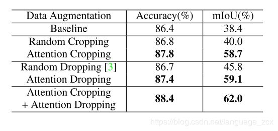
Random image cropping, is low-efficiency and a high percentage of them contain many background noises, which might lower the training efficiency, affect the quality of the extracted features and cancel out its benefits. Using Attention as guideline, the crop images may focus more on the target.
Augmentation Map
For each training image, they randomly choose one of its attention map A k A_{k} Ak to guide the data augmentation process, and normalize it as k t h k_{th} kth Augmentation Map A k ∗ A_{k}^{*} Ak∗
A k ∗ = A k − m i n ( A k ) m a x ( A k ) − m i n ( A k ) (7) A_{k}^{*} = \frac{A_{k}-min(A_{k})}{max(A_{k})-min(A_{k})} \tag{7} Ak∗=max(Ak)−min(Ak)Ak−min(Ak)(7)
Attention Cropping
Crop Mask C k C_{k} Ck from A k ∗ A_{k}^{*} Ak∗ by setting element A k ∗ ( i , j ) A_{k}^{*}(i,j) Ak∗(i,j) which is greater than threshold θ c \theta_{c} θc to 1, and others to 0, as represented in Equ 8.
C k ( i , j ) = { 1 , if A k ∗ ( i , j ) > θ c 0 , otherwise. (8) C_{k}(i,j)={\begin{cases} 1, & \text{ if } A_{k}^{*}(i,j) > \theta_{c} \\ 0, & \text {otherwise.} \end{cases}} \tag{8} Ck(i,j)={1,0, if Ak∗(i,j)>θcotherwise.(8)
We then find a bounding box Bk that can cover the whole
selected positive region of C k C_{k} Ck and enlarge this region from raw image as the augmented input data.

Attention Dropping
To encourage attention maps represent multiple discriminative object’s parts, they propose attention dropping. Specifically, they obtain attention Drop Mask D k D_{k} Dk by setting element A k ∗ ( i , j ) A_{k}^{*}(i,j) Ak∗(i,j) which is greater than threshold θ d \theta_{d} θd to 0, and others to 1, as shown in Equ 9
D k ( i , j ) = { 1 , if A k ∗ ( i , j ) > θ d 0 , otherwise. (9) D_{k}(i,j)={\begin{cases} 1, & \text{ if } A_{k}^{*}(i,j) > \theta_{d} \\ 0, & \text {otherwise.} \end{cases}} \tag{9} Dk(i,j)={1,0, if Ak∗(i,j)>θdotherwise.(9)
Object Localization and Refinement
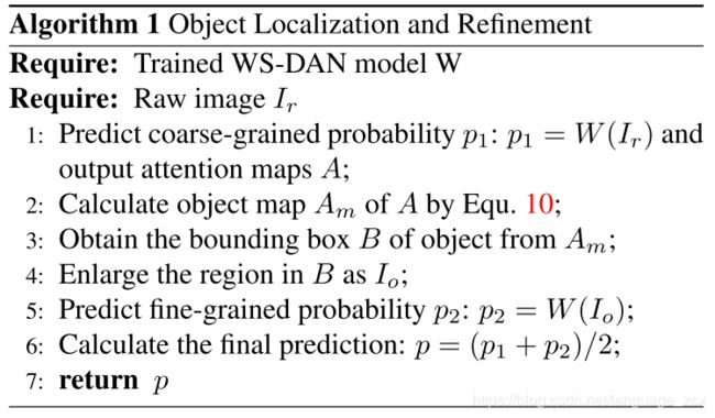
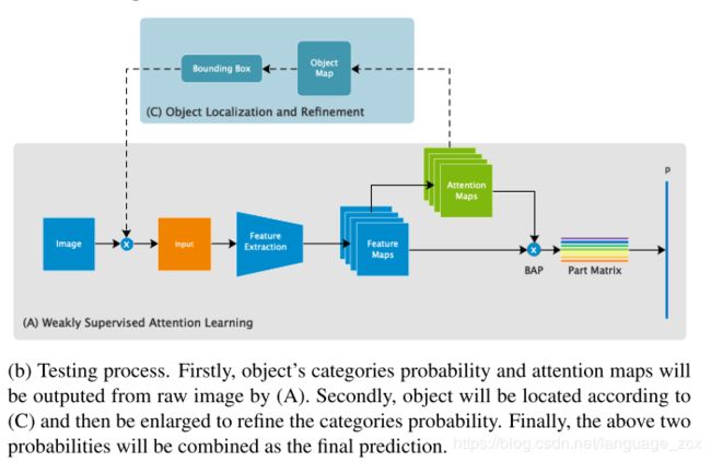
In the testing process, after the model outputs the coarse-stage classification result and corresponding attention maps for the raw image, we can predict the whole region of the object and enlarge it to predict fine-grained result by the same network model. Object Map A m A_{m} Am that indicates the location of object is calculated by Equ 10.
A m = 1 M ∑ k = 1 M A k (10) A_{m}=\frac{1}{M}\sum_{k=1}^{M} A_{k} \tag{10} Am=M1k=1∑MAk(10)
The final classification result is averaged by the coarse- grained prediction and fine-grained prediction. The detailed process of Coarse-to-Fine prediction is described as Algorithm below:
