Tensorflow2.0 InceptionResNetV2进行叶子疾病分类

1.InceptionResNetV2网络结构

论文题目：《Inception-v4, Inception-ResNet and the Impact of Residual Connections on Learning》
论文地址：https://arxiv.org/pdf/1602.07261.pdf

InceptionResNetV2的整体结构如下图所示：

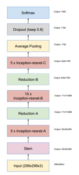
可以看到InceptionResNetV2里面的整体结构分为几个的部分
1、stem
2、Inception-resnet-A
3、Inception-resnet-B
4、Inception-resnet-C
5、Reduction-A
6、Reduction-B

其中Steam模块的结构如下：

Inception-ResNet-A的结构如下图所示：

Inception-ResNet-B的结构如下图所示：

Inception-ResNet-C的结构如下图所示：

Reduction-A的结构如下图所示：

Reduction-B的结构如下图所示：

2.数据集

链接：https://pan.baidu.com/s/1UHgrwMENNWO9PSZugW8GwA
提取码：sucd
采用kaggle上的叶子图片分类数据集，该数据集共有训练图片1820张，测试图片1820张，分别对应四个类别，即正常叶子，感染斑点病的叶子，感染锈病的叶子，感染多种疾病的叶子，这四类叶子在直观上差别不是很大，用神经网络对其进行分类有一定的难度

3.代码

#导入相应的库
from sklearn.model_selection import train_test_split
import matplotlib.pyplot as plt
from PIL import Image
import numpy as np
import pandas as pd
from tqdm import tqdm
import tensorflow as tf
import os
import cv2
tqdm.pandas()

#初始设置，设置数据集列表路径
EPOCHS = 20
SAMPLE_LEN = 600
BATCH_SIZE = 32
IMAGE_PATH = "../input/plant-pathology-2020-fgvc7/images/"
TEST_PATH = "../input/plant-pathology-2020-fgvc7/test.csv"
TRAIN_PATH = "../input/plant-pathology-2020-fgvc7/train.csv"
SUB_PATH = "../input/plant-pathology-2020-fgvc7/sample_submission.csv"

sub = pd.read_csv(SUB_PATH)
#读取测试集列表
test_data = pd.read_csv(TEST_PATH)
#读取训练集列表
train_data = pd.read_csv(TRAIN_PATH)



def load_image(image_id):
    file_path = image_id + ".jpg"
    image = cv2.imread(IMAGE_PATH + file_path)
    return cv2.cvtColor(image, cv2.COLOR_BGR2RGB)
#加载训练集前600张图片，后面进行展示
train_images = train_data["image_id"][:SAMPLE_LEN].progress_apply(load_image)


#显示数据集图片
def visualize_leaves(cond=[0, 0, 0, 0], cond_cols=["healthy"], is_cond=True):
    if not is_cond:
        cols, rows = 3, min([3, len(train_images)//3])
        fig, ax = plt.subplots(nrows=rows, ncols=cols, figsize=(30, rows*20/3))
        for col in range(cols):
            for row in range(rows):
                ax[row, col].imshow(train_images.loc[train_images.index[-row*3-col-1]])
        return None
        
    cond_0 = "healthy == {}".format(cond[0])
    cond_1 = "scab == {}".format(cond[1])
    cond_2 = "rust == {}".format(cond[2])
    cond_3 = "multiple_diseases == {}".format(cond[3])
    
    cond_list = []
    for col in cond_cols:
        if col == "healthy":
            cond_list.append(cond_0)
        if col == "scab":
            cond_list.append(cond_1)
        if col == "rust":
            cond_list.append(cond_2)
        if col == "multiple_diseases":
            cond_list.append(cond_3)
    
    data = train_data.iloc[:600]
    for cond in cond_list:
        data = data.query(cond)
        
    images = train_images.iloc[list(data.index)]
    cols, rows = 3, min([3, len(images)//3])
    
    fig, ax = plt.subplots(nrows=rows, ncols=cols, figsize=(30, rows*20/3))
    for col in range(cols):
        for row in range(rows):
            ax[row, col].imshow(images.loc[images.index[row*3+col]])
    plt.show()
    
#显示健康的叶子图片
visualize_leaves(cond=[1, 0, 0, 0], cond_cols=["healthy"])
#显示感染斑点病的叶子图片
visualize_leaves(cond=[0, 1, 0, 0], cond_cols=["scab"])
#显示感染锈病的叶子图片
visualize_leaves(cond=[0, 0, 1, 0], cond_cols=["rust"])
#显示感染多种疾病的叶子图片
visualize_leaves(cond=[0, 0, 0, 1], cond_cols=["multiple_diseases"])


def format_path(st):
    return '../input/plant-pathology-2020-fgvc7' + '/images/' + st + '.jpg'
#读取测试集图片
test_paths = test_data.image_id.apply(format_path).values
#读取训练集图片
train_paths = train_data.image_id.apply(format_path).values

#读取训练集标签
train_labels = np.float32(train_data.loc[:, 'healthy':'scab'].values)
#将训练集图片再次划分为训练集和验证集
train_paths, valid_paths, train_labels, valid_labels =train_test_split(train_paths, train_labels, test_size=0.15, random_state=2020)


#数据预处理函数
def decode_image(filename, label=None, image_size=(334, 334)):
    bits = tf.io.read_file(filename)
    image = tf.image.decode_jpeg(bits, channels=3)
    image = tf.cast(image, tf.float32) / 255.0
    image = tf.image.resize(image, image_size)
    
    if label is None:
        return image
    else:
        return image, label
#数据增强函数
def data_augment(image, label=None):
    image = tf.image.random_flip_left_right(image)
    image = tf.image.random_flip_up_down(image)
    
    if label is None:
        return image
    else:
        return image, label
#加载训练集，进行数据增强和标签打乱
train_dataset = (
     tf.data.Dataset
    .from_tensor_slices((train_paths,train_labels))
    .map(decode_image, num_parallel_calls=4)
    .map(data_augment, num_parallel_calls=4)
    .repeat()
    .shuffle(len(train_labels))
    .batch(BATCH_SIZE)
    .prefetch(1)
)
#加载验证集
valid_dataset = (
     tf.data.Dataset
    .from_tensor_slices((valid_paths, valid_labels))
    .map(decode_image, num_parallel_calls=4)
    .batch(BATCH_SIZE)
    .cache()
    .prefetch(1)
)
#加载测试集
test_dataset = (
     tf.data.Dataset
    .from_tensor_slices(test_paths)
    .map(decode_image, num_parallel_calls=4)
    .batch(BATCH_SIZE)
)


#学习率设置
def lrfn(epoch):
    LR_START = 0.00001
    LR_MAX = 0.0004
    LR_MIN = 0.00001
    LR_RAMPUP_EPOCHS = 5
    LR_SUSTAIN_EPOCHS = 0
    LR_EXP_DECAY = .8
    
    if epoch < LR_RAMPUP_EPOCHS:
        lr = (LR_MAX - LR_START) / LR_RAMPUP_EPOCHS * epoch + LR_START
    elif epoch < LR_RAMPUP_EPOCHS + LR_SUSTAIN_EPOCHS:
        lr = LR_MAX
    else:
        lr = (LR_MAX - LR_MIN) * LR_EXP_DECAY**(epoch - LR_RAMPUP_EPOCHS - LR_SUSTAIN_EPOCHS) + LR_MIN
    return lr

#绘制学习率曲线
rng = [i for i in range(EPOCHS)]
y = [lrfn(x) for x in rng]
plt.plot(rng, y)
print("Learning rate schedule: {:.3g} to {:.3g} to {:.3g}".format(y[0], max(y), y[-1]))

#构建模型
model = tf.keras.Sequential([tf.keras.applications.InceptionResNetV2(input_shape=(334,334,3),
                                             weights='imagenet',
                                             include_top=False),
                            tf.keras.layers.GlobalAveragePooling2D(),
                            tf.keras.layers.Dense(train_labels.shape[1],
                                         activation='softmax')])
#编译模型       
model.compile(optimizer='adam',
              loss = 'categorical_crossentropy',
              metrics=['accuracy'])
#打印模型参数
model.summary()

#训练参数设置
TRAIN_STEPS_PER_EPOCH = train_labels.shape[0] // BATCH_SIZE
VALID_STEPS_PER_EPOCH = valid_labels.shape[0] // BATCH_SIZE
lr_schedule = tf.keras.callbacks.LearningRateScheduler(lrfn, verbose=1)

#开始训练
history = model.fit(x=train_dataset,
                    steps_per_epoch=TRAIN_STEPS_PER_EPOCH,
                    epochs = EPOCHS,
                    validation_data=valid_dataset,
                    validation_steps=VALID_STEPS_PER_EPOCH,
                    callbacks=[lr_schedule])



# 记录准确率和损失值
history_dict = history.history
train_loss = history_dict["loss"]
train_accuracy = history_dict["accuracy"]
val_loss = history_dict["val_loss"]
val_accuracy = history_dict["val_accuracy"]

# 绘制损失值曲线
plt.figure()
plt.plot(range(EPOCHS), train_loss, label='train_loss')
plt.plot(range(EPOCHS), val_loss, label='val_loss')
plt.legend()
plt.xlabel('epochs')
plt.ylabel('loss')

# 绘制准确率曲线
plt.figure()
plt.plot(range(EPOCHS), train_accuracy, label='train_accuracy')
plt.plot(range(EPOCHS), val_accuracy, label='val_accuracy')
plt.legend()
plt.xlabel('epochs')
plt.ylabel('accuracy')
plt.show()


dict = {0:'healthy',1:'multiple_diseases',2:'rust',3:'scab'}
#获取测试集前四张图片
img = []
image = []
img1 = Image.open("../input/plant-pathology-2020-fgvc7/images/Test_0.jpg")
img.append(img1)
img2 = Image.open("../input/plant-pathology-2020-fgvc7/images/Test_1.jpg")
img.append(img2)
img3 = Image.open("../input/plant-pathology-2020-fgvc7/images/Test_2.jpg")
img.append(img3)
img4 = Image.open("../input/plant-pathology-2020-fgvc7/images/Test_3.jpg")
img.append(img4)
#将四张图片进行预测并把结果绘制出来
for i in range(0,len(img)):
    image.append(img[i])
    img[i] = img[i].resize((334,334))
    img[i] = np.array(img[i]) / 255.
    img[i] = (np.expand_dims(img[i], 0))
    result = np.squeeze(model.predict(img[i]))
    predict_class = np.argmax(result)
    plt.subplot(2,2,i+1)
    plt.title([dict[int(predict_class)],result[predict_class]])
    plt.imshow(image[i])
    plt.xticks([])
    plt.yticks([])

3.运行结果

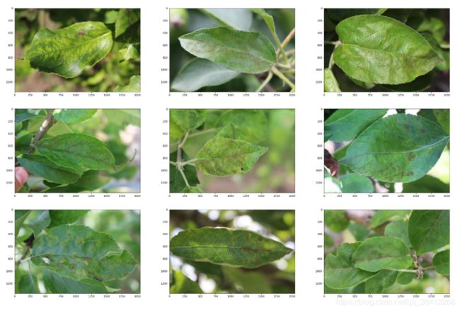
正常叶子图片

感染斑点病的叶子图片

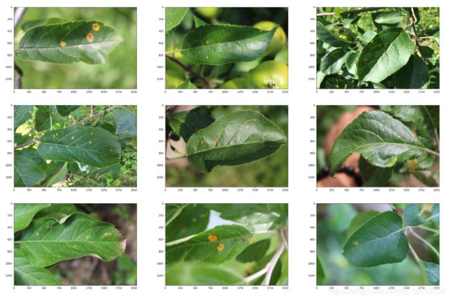
感染锈病的叶子图片

感染多种疾病的叶子图片

学习率曲线

采用余弦退火学习率，学习率会先上升再下降，上升的时候采用线性上升，下降的时候采用指数下降

模型参数

由于没有冻结其中的层，所以训练的参数量很多

Downloading data from https://storage.googleapis.com/tensorflow/keras-applications/inception_resnet_v2/inception_resnet_v2_weights_tf_dim_ordering_tf_kernels_notop.h5
219062272/219055592 [==============================] - 2s 0us/step
Model: "sequential"
_________________________________________________________________
Layer (type)                 Output Shape              Param #   
=================================================================
inception_resnet_v2 (Model)  (None, 9, 9, 1536)        54336736  
_________________________________________________________________
global_average_pooling2d (Gl (None, 1536)              0         
_________________________________________________________________
dense (Dense)                (None, 4)                 6148      
=================================================================
Total params: 54,342,884
Trainable params: 54,282,340
Non-trainable params: 60,544
_________________________________________________________________

训练过程

经过20轮训练之后验证集的准确率达到了96.48%

Epoch 00001: LearningRateScheduler reducing learning rate to 1e-05.
Epoch 1/20
48/48 [==============================] - 53s 1s/step - loss: 1.1109 - accuracy: 0.5742 - val_loss: 0.9354 - val_accuracy: 0.6836 - lr: 1.0000e-05

Epoch 00002: LearningRateScheduler reducing learning rate to 8.8e-05.
Epoch 2/20
48/48 [==============================] - 48s 999ms/step - loss: 0.3600 - accuracy: 0.8893 - val_loss: 0.2918 - val_accuracy: 0.8711 - lr: 8.8000e-05

Epoch 00003: LearningRateScheduler reducing learning rate to 0.000166.
Epoch 3/20
48/48 [==============================] - 48s 997ms/step - loss: 0.1848 - accuracy: 0.9401 - val_loss: 0.3116 - val_accuracy: 0.9141 - lr: 1.6600e-04

Epoch 00004: LearningRateScheduler reducing learning rate to 0.000244.
Epoch 4/20
48/48 [==============================] - 48s 992ms/step - loss: 0.1565 - accuracy: 0.9564 - val_loss: 0.4191 - val_accuracy: 0.9062 - lr: 2.4400e-04

Epoch 00005: LearningRateScheduler reducing learning rate to 0.000322.
Epoch 5/20
48/48 [==============================] - 48s 998ms/step - loss: 0.1252 - accuracy: 0.9596 - val_loss: 2.4625 - val_accuracy: 0.7891 - lr: 3.2200e-04

Epoch 00006: LearningRateScheduler reducing learning rate to 0.0004.
Epoch 6/20
48/48 [==============================] - 47s 983ms/step - loss: 0.1278 - accuracy: 0.9609 - val_loss: 0.5333 - val_accuracy: 0.8555 - lr: 4.0000e-04

Epoch 00007: LearningRateScheduler reducing learning rate to 0.000322.
Epoch 7/20
48/48 [==============================] - 47s 984ms/step - loss: 0.0971 - accuracy: 0.9681 - val_loss: 1.4467 - val_accuracy: 0.8477 - lr: 3.2200e-04

Epoch 00008: LearningRateScheduler reducing learning rate to 0.0002596000000000001.
Epoch 8/20
48/48 [==============================] - 48s 995ms/step - loss: 0.0592 - accuracy: 0.9824 - val_loss: 0.2279 - val_accuracy: 0.9375 - lr: 2.5960e-04

Epoch 00009: LearningRateScheduler reducing learning rate to 0.00020968000000000004.
Epoch 9/20
48/48 [==============================] - 48s 991ms/step - loss: 0.0304 - accuracy: 0.9889 - val_loss: 0.2230 - val_accuracy: 0.9453 - lr: 2.0968e-04

Epoch 00010: LearningRateScheduler reducing learning rate to 0.00016974400000000002.
Epoch 10/20
48/48 [==============================] - 48s 1s/step - loss: 0.0142 - accuracy: 0.9961 - val_loss: 0.2490 - val_accuracy: 0.9531 - lr: 1.6974e-04

Epoch 00011: LearningRateScheduler reducing learning rate to 0.00013779520000000003.
Epoch 11/20
48/48 [==============================] - 47s 980ms/step - loss: 0.0259 - accuracy: 0.9896 - val_loss: 0.1769 - val_accuracy: 0.9570 - lr: 1.3780e-04

Epoch 00012: LearningRateScheduler reducing learning rate to 0.00011223616000000004.
Epoch 12/20
48/48 [==============================] - 47s 981ms/step - loss: 0.0109 - accuracy: 0.9980 - val_loss: 0.1816 - val_accuracy: 0.9609 - lr: 1.1224e-04

Epoch 00013: LearningRateScheduler reducing learning rate to 9.178892800000003e-05.
Epoch 13/20
48/48 [==============================] - 48s 995ms/step - loss: 0.0093 - accuracy: 0.9974 - val_loss: 0.1864 - val_accuracy: 0.9688 - lr: 9.1789e-05

Epoch 00014: LearningRateScheduler reducing learning rate to 7.543114240000003e-05.
Epoch 14/20
48/48 [==============================] - 48s 1s/step - loss: 0.0025 - accuracy: 1.0000 - val_loss: 0.1817 - val_accuracy: 0.9648 - lr: 7.5431e-05

Epoch 00015: LearningRateScheduler reducing learning rate to 6.234491392000002e-05.
Epoch 15/20
48/48 [==============================] - 48s 992ms/step - loss: 0.0019 - accuracy: 1.0000 - val_loss: 0.1868 - val_accuracy: 0.9609 - lr: 6.2345e-05

Epoch 00016: LearningRateScheduler reducing learning rate to 5.1875931136000024e-05.
Epoch 16/20
48/48 [==============================] - 47s 978ms/step - loss: 0.0018 - accuracy: 1.0000 - val_loss: 0.1858 - val_accuracy: 0.9570 - lr: 5.1876e-05

Epoch 00017: LearningRateScheduler reducing learning rate to 4.3500744908800015e-05.
Epoch 17/20
48/48 [==============================] - 48s 1s/step - loss: 0.0019 - accuracy: 1.0000 - val_loss: 0.1872 - val_accuracy: 0.9609 - lr: 4.3501e-05

Epoch 00018: LearningRateScheduler reducing learning rate to 3.6800595927040014e-05.
Epoch 18/20
48/48 [==============================] - 47s 986ms/step - loss: 0.0011 - accuracy: 1.0000 - val_loss: 0.1881 - val_accuracy: 0.9609 - lr: 3.6801e-05

Epoch 00019: LearningRateScheduler reducing learning rate to 3.1440476741632015e-05.
Epoch 19/20
48/48 [==============================] - 47s 985ms/step - loss: 0.0012 - accuracy: 1.0000 - val_loss: 0.1905 - val_accuracy: 0.9648 - lr: 3.1440e-05

Epoch 00020: LearningRateScheduler reducing learning rate to 2.7152381393305616e-05.
Epoch 20/20
48/48 [==============================] - 48s 990ms/step - loss: 0.0018 - accuracy: 1.0000 - val_loss: 0.1878 - val_accuracy: 0.9648 - lr: 2.7152e-05

损失值曲线

记录每个epoch的损失值

准确率曲线

记录每个epoch的准确率

图片预测

将测试集前四张预测结果显示出来