- 机器学习knnlearn1
XW-ABAP
机器学习机器学习人工智能
importmatplotlib.pyplotaspltimportnumpyasnpimportoperator#定义一个函数用于创建数据集defcreateDataSet():#定义特征矩阵,每个元素是一个二维坐标点,代表不同策略数据点的坐标group=np.array([[20,3],[15,5],[18,1],[5,17],[2,15],[3,20]])#定义每个数据点对应的标签,用于区分
- 基于 MySQL 和 Spring Boot 的在线论坛管理系统设计与实现
城南|阿洋-计算机从小白到大神
mysqlspringboot数据库
markdownCopy✌全网粉丝20W+,csdn特邀作者、博客专家、CSDN[新星计划]导师、java领域优质创作者,博客之星、掘金/华为云/阿里云/InfoQ等平台优质作者、专注于Java、pyhton、机器学习技术领域和毕业项目实战✌哈喽兄弟们,好久不见哦~最近整理了一下之前写过的一些小项目/毕业设计。发现还是有很多存货的,想一想既然放在电脑里面也吃灰,那么还不如分享出去,没准还可以帮助到
- 零基础入门机器学习:用Scikit-learn实现鸢尾花分类
藍海琴泉
机器学习scikit-learn分类
适合人群:机器学习新手|数据分析爱好者|需快速展示案例的学生一、引言:为什么要学这个案例?目的:明确机器学习解决什么问题,建立学习信心。机器学习定义:让计算机从数据中自动学习规律(如分类鸢尾花品种)。为什么选鸢尾花数据集:数据量小、特征明确,适合教学演示。Scikit-learn优势:提供现成算法和工具,无需从头写数学公式。二、环境准备:5分钟快速上手目的:搭建可运行的代码环境,避免卡在工具安装环
- 机器学习--DBSCAN聚类算法详解
2201_75491841
机器学习算法聚类人工智能
目录引言1.什么是DBSCAN聚类?2.DBSCAN聚类算法的原理3.DBSCAN算法的核心概念3.1邻域(Neighborhood)3.2核心点(CorePoint)3.3直接密度可达(DirectlyDensity-Reachable)3.4密度可达(Density-Reachable)3.5密度相连(Density-Connected)4.DBSCAN算法的步骤5.DBSCAN算法的优缺点5
- 【机器学习】机器学习工程实战-第3章 数据收集和准备
腊肉芥末果
机器学习工程实战机器学习人工智能
上一章:第2章项目开始前文章目录3.1关于数据的问题3.1.1数据是否可获得3.1.2数据是否相当大3.1.3数据是否可用3.1.4数据是否可理解3.1.5数据是否可靠3.2数据的常见问题3.2.1高成本3.2.2质量差3.2.3噪声(noise)3.2.4偏差(bias)3.2.5预测能力低(lowpredictivepower)3.2.6过时的样本3.2.7离群值3.2.8数据泄露/目标泄漏3
- 机器学习实战 第一章 机器学习基础
LuoY、
MachineLearning机器学习算法人工智能
第一章机器学习1.1何谓机器学习1.2关键术语1.3机器学习的主要任务1.4如何选择合适的算法1.5开发机器学习应用程序的步骤1.6Python语言的优势1.1何谓机器学习 1、简单地说,机器学习就是把无序的数据转换成有用的信息; 2、机器学习能让我们自数据集中受启发,我们会利用计算机来彰显数据背后的真实含义; 3、机器学习横跨计算机科学、工程技术和统计学等多个学科,需要多学科的
- 数据挖掘实战-基于机器学习的垃圾邮件检测模型
艾派森
数据挖掘实战合集数据挖掘机器学习人工智能python
♂️个人主页:@艾派森的个人主页✍作者简介:Python学习者希望大家多多支持,我们一起进步!如果文章对你有帮助的话,欢迎评论点赞收藏加关注+目录1.项目背景2.数据集介绍
- 集成学习(随机森林)
herry57
数学建模大数据随机森林集成学习
目录一、集成学习概念二、Bagging集成原理三、随机森林四、例子(商品分类)一、集成学习概念集成学习通过建⽴⼏个模型来解决单⼀预测问题。它的⼯作原理是⽣成多个分类器/模型,各⾃独⽴地学习和作出预测。这些预测最后结合成组合预测,因此优于任何⼀个单分类的做出预测。只要单分类器的表现不太差,集成学习的结果总是要好于单分类器的二、Bagging集成原理分类圆形和长方形三、随机森林在机器学习中,随机森林是
- 【机器学习】朴素贝叶斯入门:从零到垃圾邮件过滤实战
吴师兄大模型
0基础实现机器学习入门到精通机器学习人工智能朴素贝叶斯深度学习pytorchsklearn开发语言
Langchain系列文章目录01-玩转LangChain:从模型调用到Prompt模板与输出解析的完整指南02-玩转LangChainMemory模块:四种记忆类型详解及应用场景全覆盖03-全面掌握LangChain:从核心链条构建到动态任务分配的实战指南04-玩转LangChain:从文档加载到高效问答系统构建的全程实战05-玩转LangChain:深度评估问答系统的三种高效方法(示例生成、手
- 【机器学习】机器学习工程实战-第2章 项目开始前
腊肉芥末果
机器学习工程实战机器学习人工智能
上一章:第1章概述文章目录2.1机器学习项目的优先级排序2.1.1机器学习的影响2.1.2机器学习的成本2.2估计机器学习项目的复杂度2.2.1未知因素2.2.2简化问题2.2.3非线性进展2.3确定机器学习项目的目标2.3.1模型能做什么2.3.2成功模型的属性2.4构建机器学习团队2.4.1两种文化2.4.2机器学习团队的成员2.5机器学习项目为何失败2.5.1缺乏有经验的人才2.5.2缺乏领
- 机器学习怎么做特征工程
全栈你个大西瓜
人工智能机器学习人工智能特征工程数据预处理特征变换特征降维特征构造
一、特征工程通俗解释特征工程就像厨师做菜前的食材处理:原始数据是“生肉和蔬菜”,特征工程是“切块、腌制、调料搭配”,目的是让机器学习模型(食客)更容易消化吸收,做出更好预测(品尝美味)。二、为什么要做特征工程?数据质量差:原始数据常有缺失、噪声、不一致问题(如年龄列混入“未知”)。模型限制:算法无法直接理解原始数据(如文本、日期需要数值化)。提升效果:好特征能显著提升模型性能(准确率提升10%~5
- 【机器学习】机器学习四大分类
藓类少女
机器学习机器学习分类人工智能
机器学习的方法主要可以分为四大类,根据学习方式和数据标注情况进行分类:1.监督学习(SupervisedLearning)特点:有标注数据(即训练数据有明确的输入(X)和输出(Y))。学习目标是找到一个映射(f(X)\approxY)。适用于分类和回归问题。主要算法:分类(Classification):逻辑回归(LogisticRegression)支持向量机(SVM)朴素贝叶斯(NaïveBa
- 机器学习——KNN超参数
练习AI两年半
机器学习人工智能深度学习
sklearn.model_selection.GridSearchCV是scikit-learn中用于超参数调优的核心工具,通过结合交叉验证和网格搜索实现模型参数的自动化优化。以下是详细介绍:一、功能概述GridSearchCV在指定参数网格上穷举所有可能的超参数组合,通过交叉验证评估每组参数的性能,最终选择最优参数组合。其核心价值在于:自动化调参:替代手动参数调试,提升效率3。交叉验证支持:通
- 重要重要!!fisher矩阵是怎么计算和更新的,以及计算过程中参数的物理含义
ZhangJiQun&MXP
教学2021论文2024大模型以及算力矩阵概率论线性代数windows微信机器学习
fisher矩阵是怎么计算和更新的,以及计算过程中参数的物理含义Fisher信息矩阵(FisherInformationMatrix,FIM)用于衡量模型参数估计的不确定性,其计算和更新在统计学、机器学习和优化中具有重要作用。以下是其计算和更新的关键步骤:一、Fisher矩阵的计算定义Fisher矩阵的元素表示对数似然函数关于参数的二阶导数的期望值的负数,即:Fi,j=−
- 景联文科技提供高质量文本标注服务,驱动AI技术发展
景联文科技
科技人工智能
文本标注是指在原始文本数据上添加标签的过程,这些标签可以用来指示特定的实体、关系、事件等信息,以帮助计算机理解和处理这些数据。文本标注是自然语言处理(NLP)领域的一个重要环节,它通过为文本的不同部分提供具体的含义和上下文信息,增强机器学习和深度学习模型对文本内容的理解能力。标注类型情感分析情感极性:确定文本表达的情感倾向,如正面、负面或中立。强度评估:衡量情感的强烈程度,从轻微到极端不等。命名实
- 景联文科技:以高质量数据标注推动人工智能领域创新与发展
景联文科技
科技人工智能数据标注
在当今这个由数据驱动的时代,高质量的数据标注对于推动机器学习、自然语言处理(NLP)、计算机视觉等领域的发展具有不可替代的重要性。数据标注过程涉及对原始数据进行加工,通过标注特定对象的特征来生成能够被机器学习模型识别和使用的编码格式,从而使数据更具有意义和可解读性。数据标注的主要类型包括:图像标注:指在图片中标识出目标物体的位置、形状或类别等信息,如自动驾驶技术中的行人、车辆及交通标志的识别。文本
- 客服机器人怎么才能精准的回答用户问题?
玩人工智能的辣条哥
AI面试机器人客服机器人
环境:客服机器人问题描述:客服机器人怎么才能精准的回答用户问题?解决方案:客服机器人要精准回答用户问题,需综合技术、数据和用户体验等多方面因素。以下是关键策略和步骤:1.精准理解用户意图自然语言处理(NLP)技术分词与实体识别:提取关键词(如“订单号”“退货”)和实体(如时间、地点)。意图分类:通过机器学习模型(如BERT、Transformer)将问题归类(如“售后”“支付”)。上下文理解记录对
- OpenCV 4.2.0与扩展模块安装与应用指南
土城三富
本文还有配套的精品资源,点击获取简介:OpenCV4.2.0是一个先进的计算机视觉库,包含了图像处理、计算机视觉和机器学习算法。本压缩包包含OpenCV核心库和扩展模块(opencv_contrib),版本均为4.2.0。该版本引入了性能增强、API优化以及对深度学习框架和硬件加速技术的更新支持。扩展模块提供了额外的实验性算法和功能,有助于研究和开发新算法。指南详细介绍了如何安装和配置这些库,并提
- OpenCV ML 模块使用指南
ice_junjun
OpenCVopencv人工智能计算机视觉
一、模块概述OpenCV的ML模块提供了丰富的机器学习算法,可用于解决各种计算机视觉和数据分析问题。本指南将详细介绍该模块中主要的机器学习算法,包括支持向量机(SVM)、K均值聚类(K-Means)和神经网络(ANN),并结合图像分类和聚类分析这两个典型应用场景进行代码实现与解释。二、主要函数及类详解(一)支持向量机(SVM):cv.ml.SVM_create()功能支持向量机(SVM)是一种强大
- 强化学习中策略网络模型设计与优化技巧
数字扫地僧
计算机视觉深度学习
I.引言强化学习(ReinforcementLearning,RL)是一种通过与环境交互,学习如何采取行动以最大化累积奖励的机器学习方法。策略网络(PolicyNetwork)是强化学习中一种重要的模型,它直接输出动作的概率分布或具体的动作。本篇博客将深入探讨策略网络的设计原则、优化技巧,并结合具体实例展示其应用。II.策略网络的基本概念A.策略网络的定义策略网络是一种神经网络,它接受当前状态作为
- 基于Python编程语言实现“机器学习”,用于车牌识别项目
我的sun&shine
Pythonpython机器学习计算机视觉
基于Python的验证码识别研究与实现1.摘要验证码的主要目的是区分人类和计算机,用来防止自动化脚本程序对网站的一些恶意行为,目前绝大部分网站都利用验证码来阻止恶意脚本程序的入侵。验证码的自动识别对于减少自动登录时长,识别难以识别的验证码图片有着重要的作用。对验证码图像进行灰度化、二值化、去离散噪声、字符分割、归一化、特征提取、训练和字符识别等过程可以实现验证码自动识别。首先将原图片进行灰度化处理
- DS/ML:数据科学技术之数据科学生命周期(四大层次+机器学习六大阶段+数据挖掘【5+6+6+4+4+1】步骤)的全流程最强学习路线讲解之详细攻略
一个处女座的程序猿
资深文章(前沿/经验/创新)DataScienceML数据科学数据科学的生命周期机器学习
DS/ML:数据科学技术之数据科学生命周期(四大层次+机器学习六大阶段+数据挖掘【5+6+6+4+4+1】步骤)的全流程最强学习路线讲解之详细攻略导读:本文章是博主在数据科学和机器学习领域,先后实战过几百个应用案例之后的精心总结,应该是完全覆盖了数据科学的整个生命周期及其各个阶段的要点。其中机器学习领域六大阶段更是在整个数据科学生命周期中扮演着极其重要的角色。同时,因为涉及到博主出书中出版社要求在
- 给普通人看的深度学习说明书:用快递系统理解AI如何思考
嵌入式Jerry
PythonAI人工智能深度学习
第一章:理解AI的思维方式(快递版)1.1快递分拣站的故事假设你管理一个快递分拣站:传统方法:手动制定规则(比如根据邮编分拣)机器学习:观察老员工的分拣记录,总结规律深度学习:搭建自动分拣流水线,自主发现隐藏规则1.2神经网络就像智能分拣机传送带(输入层):接收包裹信息(图片像素/文字等)#就像扫描快递单input_data=[0.2,0.7,0.1]#归一化后的特征数据分拣工人(隐藏层):每个工
- 简单理解机器学习中top_k、top_p、temperature三个参数的作用
无级程序员
机器学习人工智能
在机器学习中,top_k、top_p和temperature是用于控制生成模型(如语言模型)输出质量的参数,尤其在文本生成任务中常见。然而,网上文章很多很全,但大多晦涩难懂,今天我们来用最简单的语言谈谈它们的具体作用:1.点菜式筛选法:top_k参数英文全称:top-k中文名称:前k个具体意义:top_k参数就像是你在餐厅点菜时,服务员只给你推荐菜单上前k名的招牌菜。在AI文本生成中,top_k参
- 小白零基础学数学建模系列-引言与课程目录
川川菜鸟
数学建模小白到精通系列数学建模
目录引言一、我们的专辑包含哪些内容?第一周:数学建模基础与工具第二周:高级数学建模技巧与应用第三周:机器学习基础与数据处理第四周:监督学习与无监督学习算法第五周:神经网络二、学完本专辑能收获到什么?三、适合什么样的人群学习?四、如何学习本专辑?课程目录第1周:数学建模基础与工具第1天:数学建模入门介绍第2天:数学建模工具介绍第3天:线性回归与曲线拟合第4天:线性规划第5天:动态规划第2周:高级数学
- 初始OpenCV
指尖下的技术
OpenCVopencv人工智能计算机视觉
OpenCV是一个功能强大、应用广泛的计算机视觉库,它为开发人员提供了丰富的工具和算法,可以帮助他们快速构建各种视觉应用。随着计算机视觉技术的不断发展,OpenCV也将会继续发挥重要的作用。OpenCV提供了大量的计算机视觉算法和图像处理工具,广泛应用于图像和视频的处理、分析以及机器学习领域。所以学习人计算机视觉或者图像处理方面的知识,OpenCV是一个要重点学习的工具库。首先介绍一下OpenCV
- 机器学习结合伏羲模型高精度多尺度气象分析与降尺度实现
Hardess-god
WRF算法人工智能
随着人工智能的发展,机器学习技术在气象预报领域展现出巨大潜力。本文详细探讨如何结合机器学习(ML)和伏羲模型进行高精度多尺度气象模拟分析,并提供详细的实现步骤和相关代码。1.研究目标与技术路线目标:结合机器学习模型与伏羲气象模式,实现区域和局地高精度降尺度。技术路线:伏羲模型提供大尺度气象数据和预报使用机器学习模型(如CNN、LSTM、XGBoost)进行降尺度2.数据准备与处理2.1气象数据获取
- 基于ChatGPT、GIS与Python机器学习的地质灾害风险评估、易发性分析、信息化建库及灾后重建高级实践
weixin_贾
防洪评价风险评估滑坡泥石流地质灾害
第一章、ChatGPT、DeepSeek大语言模型提示词与地质灾害基础及平台介绍【基础实践篇】1、什么是大模型?大模型(LargeLanguageModel,LLM)是一种基于深度学习技术的大规模自然语言处理模型。代表性大模型:GPT-4、BERT、T5、ChatGPT等。特点:多任务能力:可以完成文本生成、分类、翻译、问答等任务。上下文理解:能理解复杂的上下文信息。广泛适配性:适合科研、教育、行
- 人脸识别的一些代码
饿了就干饭
CV相关人脸识别
1、cv2入门函数imread及其相关操作2、(详解)opencv里的cv2.resize改变图片大小Python3、机器学习之人脸识别face_recognition使用4、使用face_recognition进行人脸校准5、简单的人脸识别通用流程示意图(这个看着写的挺好的)6、face_recognition和图像处理中left、top、right、bottom解释7、使用pillow库对图片
- 探索Python中的集成方法:Stacking
Echo_Wish
Python笔记Python算法python开发语言
在机器学习领域,Stacking是一种高级的集成学习方法,它通过将多个基本模型的预测结果作为新的特征输入到一个元模型中,从而提高整体模型的性能和鲁棒性。本文将深入介绍Stacking的原理、实现方式以及如何在Python中应用。什么是Stacking?Stacking,又称为堆叠泛化(StackedGeneralization),是一种模型集成方法,与Bagging和Boosting不同,它并不直
- Algorithm
香水浓
javaAlgorithm
冒泡排序
public static void sort(Integer[] param) {
for (int i = param.length - 1; i > 0; i--) {
for (int j = 0; j < i; j++) {
int current = param[j];
int next = param[j + 1];
- mongoDB 复杂查询表达式
开窍的石头
mongodb
1:count
Pg: db.user.find().count();
统计多少条数据
2:不等于$ne
Pg: db.user.find({_id:{$ne:3}},{name:1,sex:1,_id:0});
查询id不等于3的数据。
3:大于$gt $gte(大于等于)
&n
- Jboss Java heap space异常解决方法, jboss OutOfMemoryError : PermGen space
0624chenhong
jvmjboss
转自
http://blog.csdn.net/zou274/article/details/5552630
解决办法:
window->preferences->java->installed jres->edit jre
把default vm arguments 的参数设为-Xms64m -Xmx512m
----------------
- 文件上传 下载 解析 相对路径
不懂事的小屁孩
文件上传
有点坑吧,弄这么一个简单的东西弄了一天多,身边还有大神指导着,网上各种百度着。
下面总结一下遇到的问题:
文件上传,在页面上传的时候,不要想着去操作绝对路径,浏览器会对客户端的信息进行保护,避免用户信息收到攻击。
在上传图片,或者文件时,使用form表单来操作。
前台通过form表单传输一个流到后台,而不是ajax传递参数到后台,代码如下:
<form action=&
- 怎么实现qq空间批量点赞
换个号韩国红果果
qq
纯粹为了好玩!!
逻辑很简单
1 打开浏览器console;输入以下代码。
先上添加赞的代码
var tools={};
//添加所有赞
function init(){
document.body.scrollTop=10000;
setTimeout(function(){document.body.scrollTop=0;},2000);//加
- 判断是否为中文
灵静志远
中文
方法一:
public class Zhidao {
public static void main(String args[]) {
String s = "sdf灭礌 kjl d{';\fdsjlk是";
int n=0;
for(int i=0; i<s.length(); i++) {
n = (int)s.charAt(i);
if((
- 一个电话面试后总结
a-john
面试
今天,接了一个电话面试,对于还是初学者的我来说,紧张了半天。
面试的问题分了层次,对于一类问题,由简到难。自己觉得回答不好的地方作了一下总结:
在谈到集合类的时候,举几个常用的集合类,想都没想,直接说了list,map。
然后对list和map分别举几个类型:
list方面:ArrayList,LinkedList。在谈到他们的区别时,愣住了
- MSSQL中Escape转义的使用
aijuans
MSSQL
IF OBJECT_ID('tempdb..#ABC') is not null
drop table tempdb..#ABC
create table #ABC
(
PATHNAME NVARCHAR(50)
)
insert into #ABC
SELECT N'/ABCDEFGHI'
UNION ALL SELECT N'/ABCDGAFGASASSDFA'
UNION ALL
- 一个简单的存储过程
asialee
mysql存储过程构造数据批量插入
今天要批量的生成一批测试数据,其中中间有部分数据是变化的,本来想写个程序来生成的,后来想到存储过程就可以搞定,所以随手写了一个,记录在此:
DELIMITER $$
DROP PROCEDURE IF EXISTS inse
- annot convert from HomeFragment_1 to Fragment
百合不是茶
android导包错误
创建了几个类继承Fragment, 需要将创建的类存储在ArrayList<Fragment>中; 出现不能将new 出来的对象放到队列中,原因很简单;
创建类时引入包是:import android.app.Fragment;
创建队列和对象时使用的包是:import android.support.v4.ap
- Weblogic10两种修改端口的方法
bijian1013
weblogic端口号配置管理config.xml
一.进入控制台进行修改 1.进入控制台: http://127.0.0.1:7001/console 2.展开左边树菜单 域结构->环境->服务器-->点击AdminServer(管理) &
- mysql 操作指令
征客丶
mysql
一、连接mysql
进入 mysql 的安装目录;
$ bin/mysql -p [host IP 如果是登录本地的mysql 可以不写 -p 直接 -u] -u [userName] -p
输入密码,回车,接连;
二、权限操作[如果你很了解mysql数据库后,你可以直接去修改系统表,然后用 mysql> flush privileges; 指令让权限生效]
1、赋权
mys
- 【Hive一】Hive入门
bit1129
hive
Hive安装与配置
Hive的运行需要依赖于Hadoop,因此需要首先安装Hadoop2.5.2,并且Hive的启动前需要首先启动Hadoop。
Hive安装和配置的步骤
1. 从如下地址下载Hive0.14.0
http://mirror.bit.edu.cn/apache/hive/
2.解压hive,在系统变
- ajax 三种提交请求的方法
BlueSkator
Ajaxjqery
1、ajax 提交请求
$.ajax({
type:"post",
url : "${ctx}/front/Hotel/getAllHotelByAjax.do",
dataType : "json",
success : function(result) {
try {
for(v
- mongodb开发环境下的搭建入门
braveCS
运维
linux下安装mongodb
1)官网下载mongodb-linux-x86_64-rhel62-3.0.4.gz
2)linux 解压
gzip -d mongodb-linux-x86_64-rhel62-3.0.4.gz;
mv mongodb-linux-x86_64-rhel62-3.0.4 mongodb-linux-x86_64-rhel62-
- 编程之美-最短摘要的生成
bylijinnan
java数据结构算法编程之美
import java.util.HashMap;
import java.util.Map;
import java.util.Map.Entry;
public class ShortestAbstract {
/**
* 编程之美 最短摘要的生成
* 扫描过程始终保持一个[pBegin,pEnd]的range,初始化确保[pBegin,pEnd]的ran
- json数据解析及typeof
chengxuyuancsdn
jstypeofjson解析
// json格式
var people='{"authors": [{"firstName": "AAA","lastName": "BBB"},'
+' {"firstName": "CCC&
- 流程系统设计的层次和目标
comsci
设计模式数据结构sql框架脚本
流程系统设计的层次和目标
- RMAN List和report 命令
daizj
oraclelistreportrman
LIST 命令
使用RMAN LIST 命令显示有关资料档案库中记录的备份集、代理副本和映像副本的
信息。使用此命令可列出:
• RMAN 资料档案库中状态不是AVAILABLE 的备份和副本
• 可用的且可以用于还原操作的数据文件备份和副本
• 备份集和副本,其中包含指定数据文件列表或指定表空间的备份
• 包含指定名称或范围的所有归档日志备份的备份集和副本
• 由标记、完成时间、可
- 二叉树:红黑树
dieslrae
二叉树
红黑树是一种自平衡的二叉树,它的查找,插入,删除操作时间复杂度皆为O(logN),不会出现普通二叉搜索树在最差情况时时间复杂度会变为O(N)的问题.
红黑树必须遵循红黑规则,规则如下
1、每个节点不是红就是黑。 2、根总是黑的 &
- C语言homework3,7个小题目的代码
dcj3sjt126com
c
1、打印100以内的所有奇数。
# include <stdio.h>
int main(void)
{
int i;
for (i=1; i<=100; i++)
{
if (i%2 != 0)
printf("%d ", i);
}
return 0;
}
2、从键盘上输入10个整数,
- 自定义按钮, 图片在上, 文字在下, 居中显示
dcj3sjt126com
自定义
#import <UIKit/UIKit.h>
@interface MyButton : UIButton
-(void)setFrame:(CGRect)frame ImageName:(NSString*)imageName Target:(id)target Action:(SEL)action Title:(NSString*)title Font:(CGFloa
- MySQL查询语句练习题,测试足够用了
flyvszhb
sqlmysql
http://blog.sina.com.cn/s/blog_767d65530101861c.html
1.创建student和score表
CREATE TABLE student (
id INT(10) NOT NULL UNIQUE PRIMARY KEY ,
name VARCHAR
- 转:MyBatis Generator 详解
happyqing
mybatis
MyBatis Generator 详解
http://blog.csdn.net/isea533/article/details/42102297
MyBatis Generator详解
http://git.oschina.net/free/Mybatis_Utils/blob/master/MybatisGeneator/MybatisGeneator.
- 让程序员少走弯路的14个忠告
jingjing0907
工作计划学习
无论是谁,在刚进入某个领域之时,有再大的雄心壮志也敌不过眼前的迷茫:不知道应该怎么做,不知道应该做什么。下面是一名软件开发人员所学到的经验,希望能对大家有所帮助
1.不要害怕在工作中学习。
只要有电脑,就可以通过电子阅读器阅读报纸和大多数书籍。如果你只是做好自己的本职工作以及分配的任务,那是学不到很多东西的。如果你盲目地要求更多的工作,也是不可能提升自己的。放
- nginx和NetScaler区别
流浪鱼
nginx
NetScaler是一个完整的包含操作系统和应用交付功能的产品,Nginx并不包含操作系统,在处理连接方面,需要依赖于操作系统,所以在并发连接数方面和防DoS攻击方面,Nginx不具备优势。
2.易用性方面差别也比较大。Nginx对管理员的水平要求比较高,参数比较多,不确定性给运营带来隐患。在NetScaler常见的配置如健康检查,HA等,在Nginx上的配置的实现相对复杂。
3.策略灵活度方
- 第11章 动画效果(下)
onestopweb
动画
index.html
<!DOCTYPE html PUBLIC "-//W3C//DTD XHTML 1.0 Transitional//EN" "http://www.w3.org/TR/xhtml1/DTD/xhtml1-transitional.dtd">
<html xmlns="http://www.w3.org/
- FAQ - SAP BW BO roadmap
blueoxygen
BOBW
http://www.sdn.sap.com/irj/boc/business-objects-for-sap-faq
Besides, I care that how to integrate tightly.
By the way, for BW consultants, please just focus on Query Designer which i
- 关于java堆内存溢出的几种情况
tomcat_oracle
javajvmjdkthread
【情况一】:
java.lang.OutOfMemoryError: Java heap space:这种是java堆内存不够,一个原因是真不够,另一个原因是程序中有死循环; 如果是java堆内存不够的话,可以通过调整JVM下面的配置来解决: <jvm-arg>-Xms3062m</jvm-arg> <jvm-arg>-Xmx
- Manifest.permission_group权限组
阿尔萨斯
Permission
结构
继承关系
public static final class Manifest.permission_group extends Object
java.lang.Object
android. Manifest.permission_group 常量
ACCOUNTS 直接通过统计管理器访问管理的统计
COST_MONEY可以用来让用户花钱但不需要通过与他们直接牵涉的权限
D

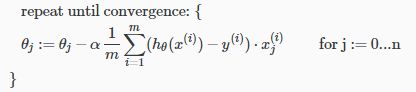
 是
是  的平均值或者是标准差
  是
是  ,可以通过绘制代价函数
  的图像来调试学习率
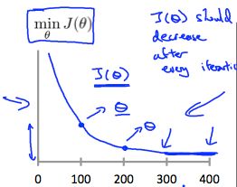
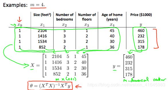
 都置为 1.