机器学习实战（基于Sklearn和tensorflow）第三章 分类 学习笔记

机器学习实战 书籍第三章例子学习笔记
书中源码，here
本文地址，here
要分为Mnist数据处理、交叉验证、混淆矩阵、精度、多分类问题等。

加载数据 可以从本地下载

fetch_mldata下载较慢，可以下载到本地
链接：https://pan.baidu.com/s/1fAInuofJ_MJJfvNjY1djsg
提取码：e462
在当前工程目录下新建并拷贝自己下载文件
datasets/mldata/mnist-original.mat
其实从fetch_mldata源码里看到 是从这个目录下加载。

from sklearn.datasets import fetch_mldata
mnist = fetch_mldata('MNIST original',data_home='./datasets')
X, y = mnist["data"], mnist["target"]

%matplotlib inline
import matplotlib
import matplotlib.pyplot as plt

some_digit = X[36000]
some_digit_image = some_digit.reshape(28, 28)
plt.imshow(some_digit_image, cmap=plt.get_cmap("binary"), interpolation="nearest")
plt.axis("off")
plt.show()

X_train, X_test, y_train, y_test = X[:60000], X[60000:], y[:60000], y[60000:]
#打乱数据
import numpy as np
shuffle_index = np.random.permutation(60000)
X_train, y_train = X_train[shuffle_index], y_train[shuffle_index]

训练一个二分类器

y_train_5 = (y_train == 5)
y_test_5 = (y_test == 5)
from sklearn.linear_model import SGDClassifier
sgd_clf = SGDClassifier(random_state=42, max_iter=5, tol=None)
sgd_clf.fit(X_train, y_train_5)
sgd_clf.predict([some_digit])

性能考核

使用交叉验证测量精度

自定义分组
分成3组 每次取一组作为验证 总共三个输出

from sklearn.model_selection import StratifiedKFold
from sklearn.base import clone

skfolds = StratifiedKFold(n_splits=3, random_state=42)
for train_index, test_index in skfolds.split(X_train, y_train_5):
    clone_clf = clone(sgd_clf)
    X_train_folds = X_train[train_index]
    y_train_folds = y_train_5[train_index]
    X_test_fold = X_train[test_index]
    y_test_fold = y_train_5[test_index]
    
    clone_clf.fit(X_train_folds, y_train_folds)
    y_pre = clone_clf.predict(X_test_fold)
    n_correct = sum(y_pre == y_test_fold)
    print(n_correct / len(y_pre))

from sklearn.model_selection import cross_val_score
cross_val_score(sgd_clf, X_train, y_train_5, cv=3, scoring="accuracy")

Never5Classifier这里返回全false 判断输入是非5 也就是输入任何数据准确率都可以达到90%

from sklearn.base import BaseEstimator
class Never5Classifier(BaseEstimator):
    def fit(self, X, y=None):
        pass
    def predict(self, X):
        return np.zeros((len(X), 1), dtype=bool)
never_5_clf = Never5Classifier()
cross_val_score(never_5_clf, X_train, y_train_5, cv=3, scoring="accuracy") 

混淆矩阵 精度 召回率

数量	预测成负样本	预测成正样本
实际是负样本	52509 TN true negatives	2070 FP false positives
实际是正样本	1118 FN false negatives	4303 TP true positives

52509表示负样本预测对了 2070表示应该是负样本，但是却预测成正样本了
1118 实际是正样本，但是预测成负样本了 4303预测正样本成功
一个完美的分类器得到混淆矩阵应该是反对角线为0：

数量	预测成负样本	预测成正样本
实际是负样本	yyyyy	0
实际是正样本	0	xxxx

分类器精度 $\frac{TP}{TP+FP}$ 即$\frac{4303}{4303+2070}$
而上一步精度是$\frac{52509+4303}{60000}=0.947$

召回率 （灵敏度或真正类TPR）
$\frac{TP}{TP+FN}$

组合召回率和精度F1
$\frac{2}{\frac{1}{精度}+\frac{1}{召回率}}$

#cross_val_predict 返回单个样本分类
from sklearn.model_selection import cross_val_predict
y_train_pred = cross_val_predict(sgd_clf, X_train, y_train_5, cv=3)
from sklearn.metrics import confusion_matrix
confusion_matrix(y_train_5, y_train_pred)

#精度 召回率 F1分数
from sklearn.metrics import precision_score, recall_score
print("precision : ", precision_score(y_train_5, y_train_pred), " recall : ", recall_score(y_train_5, y_train_pred))
from sklearn.metrics import f1_score
f1_score(y_train_5, y_train_pred)

精度/召回率权衡

cross_val_predict 获取所有训练样本分数
通过该阈值来计算所有可能阈值对应的精度和召回率

#查看样例分数
y_scores = sgd_clf.decision_function([some_digit])
#获取模型样例的分数
y_scores = cross_val_predict(sgd_clf, X_train, y_train_5, cv=3, method="decision_function")

通过观察曲线可以得到精度和召回率变化大致趋势相反
实际场景可根据曲线取得合适的值

from sklearn.metrics import precision_recall_curve
precisions, recalls, thresholds = precision_recall_curve(y_train_5, y_scores)
def plot_precision_recall_vs_threshold(precisions, recalls, thresholds):
    plt.plot(thresholds, precisions[:-1], "b--", label="Precisions")
    plt.plot(thresholds, recalls[:-1], "g-", label="Recalls")
    plt.xlabel("Threshold")
    plt.legend(loc="upper left")
    plt.ylim([0, 1])
plot_precision_recall_vs_threshold(precisions, recalls, thresholds)
plt.show()
plt.plot(precisions[:-1], recalls[:-1], 'r')
plt.xlabel("precisions")
plt.ylabel("recalls")
plt.show()

因为随机梯度下降分类器使用的阈值是0
这里使用70000 可以看到准确率提升了

y_train_pred_90 = (y_scores > 70000)
# 之前阈值为0时候 precision :  0.6751922171661697  recall :  0.7937649880095923
print("precision : ", precision_score(y_train_5, y_train_pred_90), " recall : ", recall_score(y_train_5, y_train_pred_90))

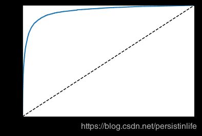
ROC曲线

ROC曲线描述的是召回率和假正类率FPR的关系
FPR=1-TNR 也就是实际负类集合中被识别成正类的比例
FPR=$\frac{FP}{FP+TN}$
TNR=$\frac{TN}{FP+TN}$
一个完美分类器ROC 曲线下面积AUC应该是1

from sklearn.metrics import roc_curve
fpr, tpr, thresholds = roc_curve(y_train_5, y_scores)
def plot_roc_curve(fpr, tpr, label=None):
    plt.plot(fpr, tpr, linewidth=2, label=label)
    plt.plot([0, 1], [0, 1], 'k--')
    plt.axis([0, 1, 0, 1])
    plt.xlabel('FPR')
    plt.ylabel('TPR')
plot_roc_curve(fpr, tpr)
plt.show()
from sklearn.metrics import roc_auc_score
roc_auc_score(y_train_5, y_scores)

训练一个随机森林分类器，对比随机梯度下降分类器

from sklearn.ensemble import RandomForestClassifier
forest_clf = RandomForestClassifier(random_state=42, n_estimators=10)
y_probas_forest = cross_val_predict(forest_clf, X_train, y_train_5, cv=3, method="predict_proba")
y_scores_forest = y_probas_forest[:, 1]
fpr_forest, tpr_forest, thresholds_forest = roc_curve(y_train_5, y_scores_forest)
plt.plot(fpr, tpr, "b:", label="SGD")
plot_roc_curve(fpr_forest, tpr_forest, "Random Forest")
plt.legend(loc="best")
plt.show()

多类别分类器

• 一对多OvA例如一个系统将数字图片分为10个类别 那么就有10个分类器
• 二元分类器OvO 例如一个区分0和1 0和2 1和2 如果存在N个分类共需要N*(N-1)/2 优点每个分类器只需要部分训练对需要区分的类别进行区分
  sklearn默认用OvA (svm例外 默认使用OvO)

sgd_clf.fit(X_train, y_train)
some_digit_scores = sgd_clf.decision_function([some_digit])
some_digit_scores

np.argmax(some_digit_scores)
sgd_clf.classes_

from sklearn.multiclass import OneVsOneClassifier
ovo_clf = OneVsOneClassifier(SGDClassifier(random_state=42, max_iter=5, tol=None))
ovo_clf.fit(X_train, y_train)
ovo_clf.predict([some_digit])

len(ovo_clf.estimators_)
cross_val_score(sgd_clf, X_train, y_train, cv=3, scoring="accuracy")

#进行缩放之后调整模型准确率 去均值和方差归一化
from sklearn.preprocessing import StandardScaler
scaler = StandardScaler()
X_train_scaled = scaler.fit_transform(X_train.astype(np.float64))
cross_val_score(sgd_clf, X_train_scaled, y_train, cv=3, scoring="accuracy")

错误分析

判断10个分类数据的混淆矩阵
由下图对角线可以看出绝大部分分类都是正确的

y_train_pred = cross_val_predict(sgd_clf, X_train_scaled, y_train, cv=3)
conf_mx = confusion_matrix(y_train, y_train_pred)
conf_mx
plt.matshow(conf_mx, cmap=plt.cm.gray)
plt.show()

#更加突出识别错误的标签
row_sums = conf_mx.sum(axis=1, keepdims=True)
norm_conf_mx = conf_mx / row_sums
np.fill_diagonal(norm_conf_mx, 0)
plt.matshow(norm_conf_mx, cmap=plt.cm.gray)
plt.show()

多标签分类

输入一个样本，输出多个纬度的分类结果
例子是分类标签是是否大于7和是否是奇数

from sklearn.neighbors import KNeighborsClassifier
y_train_large = (y_train > 7)
y_train_odd = (y_train % 2 == 1)
#
y_multilabel = np.c_[y_train_large, y_train_odd]
knn_clf = KNeighborsClassifier()
knn_clf.fit(X_train, y_multilabel)
knn_clf.predict([some_digit])

f1_score
‘macro’: 对每一类别的f1_score进行简单算术平均
‘weighted’: 对每一类别的f1_score进行加权平均，权重为各类别数在y_true中所占比例。
‘micro’: 设置average='micro’时，Precision = Recall = F1_score = Accuracy。
None：返回每一类各自的f1_score，得到一个array。
‘binary’: 只对二分类问题有效，返回由pos_label指定的类的f1_score。

y_train_knn_pred = cross_val_predict(knn_clf, X_train, y_train, cv=3)#运行时间较长
f1_score(y_train, y_train_knn_pred, average="macro")

多输出分类

多输出-多类别
例子：对原始图片增加噪点 增加噪点前数据杨输入X 标签是原始数据

# X_train_split = X_train[0:10000]
# X_test_split = X_test[0:10000]
# print(len(X_train_split))
noise_train = np.random.randint(0, 100, (len(X_train), 784))
noise_test = np.random.randint(0, 100, (len(X_test), 784))

X_tran_mod = X_train + noise_train
X_test_mod = X_test + noise_test
y_train_mod = X_train
y_test_mod = X_test

knn_clf.fit(X_tran_mod, y_train_mod)
clean_digit = knn_clf.predict([X_test_mod[2]])

some_digit_image = clean_digit.reshape(28, 28)
plt.imshow(some_digit_image, cmap=plt.get_cmap("binary"), interpolation="nearest")
plt.axis("off")
plt.show()
some_digit_image = X_test_mod[2].reshape(28, 28)
plt.imshow(some_digit_image, cmap=plt.get_cmap("binary"), interpolation="nearest")
plt.axis("off")
plt.show()