kaggle-房价预测案例

 此案例为kaggle上面的房价预测案例

https://www.kaggle.com/c/house-prices-advanced-regression-techniques

具体代码如下

import numpy as np
import pandas as pd
import matplotlib.pyplot as plt
#-------------------Step1:读取数据---------------------
train_df=pd.read_csv('C:\\Users\\Administrator\\Desktop\\network\\House_prise\\train.csv')
test_df=pd.read_csv('C:\\Users\\Administrator\\Desktop\\network\\House_prise\\test.csv')

#查看数据前5行
print(train_df.head())
print(test_df.head())
'''
   Id  MSSubClass MSZoning    ...     SaleType  SaleCondition SalePrice
0   1          60       RL    ...           WD         Normal    208500
1   2          20       RL    ...           WD         Normal    181500
2   3          60       RL    ...           WD         Normal    223500
3   4          70       RL    ...           WD        Abnorml    140000
4   5          60       RL    ...           WD         Normal    250000

[5 rows x 81 columns]
     Id  MSSubClass MSZoning      ...       YrSold  SaleType SaleCondition
0  1461          20       RH      ...         2010        WD        Normal
1  1462          20       RL      ...         2010        WD        Normal
2  1463          60       RL      ...         2010        WD        Normal
3  1464          60       RL      ...         2010        WD        Normal
4  1465         120       RL      ...         2010        WD        Normal

[5 rows x 79 columns]
'''
#-----------------------------------Step2:合并数据---------------------------------
#这么做是为了把训练集和测试集的数据一块来一次性处理，等到处理完后再将他们分开
#上面在训练集中的最后一个属性SalePrice为我们的训练目标，因此只出现在训练集中，所以我们先将它
#作为y_train拿出来

#我们先看SalePrice长什么样
prices=pd.DataFrame({'Prices':train_df['SalePrice'],'log(price+1)':np.log1p(train_df['SalePrice'])})
print(prices.hist())
plt.show()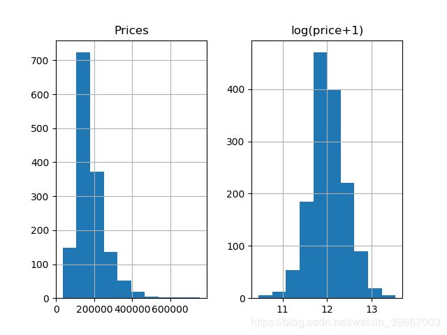

 从上图可以看出，测试集中的预测目标‘SalePrice’特征并不正态化，为了让我们的预测目标平滑一些，我们可以使用log(X+1)即log1p，所得结果如右图所示。需要注意的是，最后计算结果的时候，记得把预测到的平滑数据变回去，使用expm1().

#将train_df中的属性‘SalePrice’取出给y_train,此时train_df中就没有这一属性了
y_train=np.log1p(train_df.pop('SalePrice'))
#将剩余部分按照行合并起来
all_df=pd.concat((train_df,test_df),axis=0)
#查看合并后的形状
print(all_df.shape)
'''
(2919, 79)
'''
print(y_train.head())#查看y_train
'''
0    12.247699
1    12.109016
2    12.317171
3    11.849405
4    12.429220
Name: SalePrice, dtype: float64
'''

#-----------------------------------Step3: 变量转换-----------------------------------
#首先我们观察到'MSSubClass'的值虽然用不同的数字表示，但它应该是一些类别，我们要将它变回string类型
print(all_df['MSSubClass'].dtypes)
'''
int64
'''
all_df['MSSubClass']=all_df['MSSubClass'].astype(str)
#变成str后，做个统计就清楚了
print(all_df['MSSubClass'].value_counts())
'''
20     1079
60      575
50      287
120     182
30      139
160     128
70      128
80      118
90      109
190      61
85       48
75       23
45       18
180      17
40        6
150       1
Name: MSSubClass, dtype: int64
'''
#把category的变量转变成numerical表达形式
print(pd.get_dummies(all_df['MSSubClass'],prefix='MSSubClass').head())#此刻MSSubClass被我们分成了16个column，每一个代表一个category。是就是1，不是就是0。
'''
   MSSubClass_120  MSSubClass_150      ...        MSSubClass_85  MSSubClass_90
0               0               0      ...                    0              0
1               0               0      ...                    0              0
2               0               0      ...                    0              0
3               0               0      ...                    0              0
4               0               0      ...                    0              0

[5 rows x 16 columns]
'''
#同理，我们把所有的catagory数据都使用one-hot编码
all_dummy_df=pd.get_dummies(all_df)
print(all_dummy_df.head())
'''
   Id          ...            SaleCondition_Partial
0   1          ...                                0
1   2          ...                                0
2   3          ...                                0
3   4          ...                                0
4   5          ...                                0

[5 rows x 303 columns]
'''

#对缺失值的处理
#查看缺失值，计算每个属性的缺失值个数，将其按照从多到少排序
print(all_dummy_df.isnull().sum().sort_values(ascending=False).head(10))
'''
[5 rows x 303 columns]
LotFrontage     486
GarageYrBlt     159
MasVnrArea       23
BsmtFullBath      2
BsmtHalfBath      2
GarageCars        1
BsmtFinSF1        1
BsmtFinSF2        1
BsmtUnfSF         1
TotalBsmtSF       1
dtype: int64
'''
#可以看到，缺失最多的column是LotFrontage
#在这里，我们用平均值来填满这些空缺。
mean_cols=all_dummy_df.mean()
all_dummy_df=all_dummy_df.fillna(mean_cols)
#查看是否还有空缺值
print(all_dummy_df.isnull().sum().sum())
'''
0
'''
#标准化数据
#我们不需要把One-Hot的那些0/1数据给标准化。我们的目标是那些本来就是numerical的数据
numeric_cols=all_df.columns[all_df.dtypes!='object']
print(numeric_cols)
#计算标准分布(X-X')/S
numeric_cols_means=all_dummy_df.loc[:,numeric_cols].mean()
numeric_cols_std=all_dummy_df.loc[:,numeric_cols].std()
all_dummy_df.loc[:,numeric_cols]=(all_dummy_df.loc[:,numeric_cols]-numeric_cols_means)/numeric_cols_std

#-------------------------------Step 4:建立模型-----------------------------------------
#把数据集分回训练/测试集
dummy_train_df=all_dummy_df.loc[train_df.index]
dummy_test_df=all_dummy_df.loc[test_df.index]
print(dummy_train_df.shape,dummy_test_df.shape)
'''
(1460, 303) (1459, 303)
'''
#岭回归
#对于多因子的数据集，这种模型可以方便的把所有的var都无脑的放进去
from sklearn.linear_model import Ridge
from sklearn.model_selection import cross_val_score

#这一步不是很必要，只是把DF转化成Numpy Array，这跟Sklearn更加配
X_train=dummy_train_df.values
X_test=dummy_test_df.values

#用Sklearn自带的cross validation方法来测试模型
alphas=np.logspace(-3,2,50)
test_scores=[]
for alpha in alphas:
    clf=Ridge(alpha)
    test_score=np.sqrt(-cross_val_score(clf,X_train,y_train,cv=10,scoring='neg_mean_squared_error'))
    test_scores.append(np.mean(test_score))

#存下所有的CV值，看看哪个alpha值更好
plt.plot(alphas,test_scores)
plt.title("Alpha vs CV Error")
plt.show()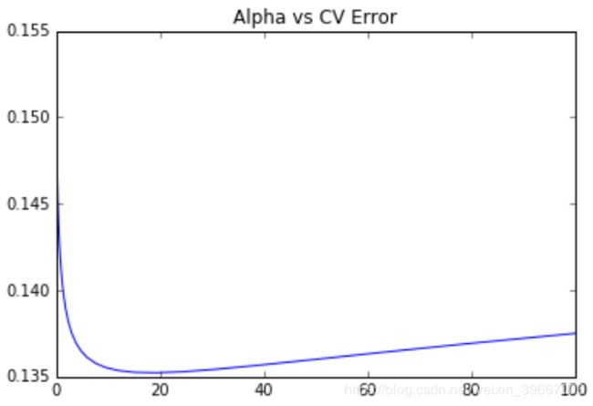

 

#随机森林
from sklearn.ensemble import RandomForestRegressor
max_features=[.1,.3,.5,.7,.9,.99]
test_scores=[]
for max_feature in max_features:
    clf=RandomForestRegressor(n_estimators=200,max_features=max_feature)
    test_score=np.sqrt(-cross_val_score(clf,X_train,y_train,cv=5,scoring='neg_mean_squared_error'))
    test_scores.append(np.mean(test_score))
plt.plot(max_features,test_scores)
plt.title('Max Features vs CV Error')
plt.show()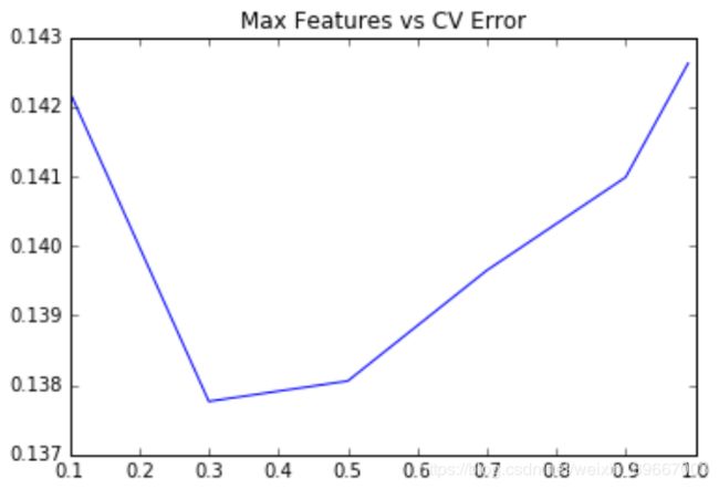

 

#--------------------------------Step5:模型融合----------------------------------
#这里我们用一个Stacking的思维来汲取两种或者多种模型的优点
#首先，我们把最好的parameter拿出来，做成我们最终的model
ridge=Ridge(alpha=15)
rf=RandomForestRegressor(n_estimators=500,max_features=.3)
ridge.fit(X_train,y_train)
rf.fit(X_train,y_train)

#上面提到了，因为最前面我们给label做了个log(1+x), 于是这里我们需要把predit的值给exp回去，并且减掉那个"1"
#所以就是我们的expm1()函数。
y_ridge=np.expm1(ridge.predict(X_test))
y_rf=np.expm1(rf.predict(X_test))

#一个正经的Ensemble是把这群model的预测结果作为新的input，再做一次预测。这里我们简单的方法，就是直接『平均化』。
y_final=(y_ridge+y_rf)/2

#-----------------------------------------Step6：提交结果--------------------------------------
submission_df=pd.DataFrame(data={'Id':test_df.index,'SalePrice':y_final})
print(submission_df.head(10))
'''
     Id      SalePrice
0  1461  118872.530547
1  1462  150845.024158
2  1463  175443.392106
3  1464  190153.672131
4  1465  195473.772773
5  1466  176301.877235
6  1467  177621.182529
7  1468  169012.173189
8  1469  184472.271054
9  1470  122613.992701
'''

 由于单个分类器效果是有限的，我们可以把N多个分类器合在一起，做一个综合分类器达到最好的效果。

#Bagging
#Bagging把很多的小分类器放在一起，每个train随机的一部分数据，然后把它们的最终结果综合起来（多数投票制）。
from sklearn.ensemble import BaggingRegressor
params = [1, 10, 15, 20, 25, 30, 40]
test_scores = []
for param in params:
    clf = BaggingRegressor(n_estimators=param, base_estimator=ridge)#使用上面的小分类器ridge
    test_score = np.sqrt(-cross_val_score(clf, X_train, y_train, cv=10, scoring='neg_mean_squared_error'))
    test_scores.append(np.mean(test_score))

plt.plot(params, test_scores)
plt.title("n_estimator vs CV Error")

#使用Bagging自带的DecisionTree模型
params = [10, 15, 20, 25, 30, 40, 50, 60, 70, 100]
test_scores = []
for param in params:
    clf = BaggingRegressor(n_estimators=param)
    test_score = np.sqrt(-cross_val_score(clf, X_train, y_train, cv=10, scoring='neg_mean_squared_error'))
    test_scores.append(np.mean(test_score))

plt.plot(params, test_scores)
plt.title("n_estimator vs CV Error")

#Boosting
#Boosting比Bagging理论上更高级点，它也是揽来一把的分类器。但是把他们线性排列。
#下一个分类器把上一个分类器分类得不好的地方加上更高的权重，这样下一个分类器就能在这个部分学得更加“深刻”。
from sklearn.ensemble import AdaBoostRegressor
params = [10, 15, 20, 25, 30, 35, 40, 45, 50]
test_scores = []
for param in params:
    clf = BaggingRegressor(n_estimators=param, base_estimator=ridge)
    test_score = np.sqrt(-cross_val_score(clf, X_train, y_train, cv=10, scoring='neg_mean_squared_error'))
    test_scores.append(np.mean(test_score))
plt.plot(params, test_scores)
plt.title("n_estimator vs CV Error")

#最后，我们来看看巨牛逼的XGBoost，外号：Kaggle神器
#这依旧是一款Boosting框架的模型，但是却做了很多的改进。
from xgboost import XGBRegressor
params=[1,2,3,4,5,6]
test_scores=[]
for param in params:
    clf=XGBRegressor(max_depth=param)
    test_score=np.sqrt(-cross_val_score(clf,X_train,y_train,cv=10,scoring='neg_mean_squared_error'))
    test_scores.append(np.mean(test_score))

plt.plot(params,test_scores)
plt.title('max_depth vs CV Error')