原文链接:http://tecdat.cn/category/大数据部落/
Objection:
We attempts to explore the relationship between different demographic factors to crime rate, find out the important factors related to crime rate and the factors that have important influence on crime rate through regression model. Finally, we summarize the model and make suggestions on the control of crime rate`
Population Income Illiteracy Life Exp Murder HS Grad Frost
Alabama 3615 3624 2.1 69.05 15.1 41.3 20
Alaska 365 6315 1.5 69.31 11.3 66.7 152
Arizona 2212 4530 1.8 70.55 7.8 58.1 15
Arkansas 2110 3378 1.9 70.66 10.1 39.9 65
California 21198 5114 1.1 71.71 10.3 62.6 20
Colorado 2541 4884 0.7 72.06 6.8 63.9 166
Area
Alabama 50708
Alaska 566432
Arizona 113417
Arkansas 51945
California 156361
Colorado 103766
`
determine the impact of the various factors on the murder rate in each state in the USA.Consider the marginal and bivariate distributions`
Population Income Illiteracy Life Exp Murder HS Grad Frost
Alabama 3615 3624 2.1 69.05 15.1 41.3 20
Alaska 365 6315 1.5 69.31 11.3 66.7 152
Arizona 2212 4530 1.8 70.55 7.8 58.1 15
Arkansas 2110 3378 1.9 70.66 10.1 39.9 65
California 21198 5114 1.1 71.71 10.3 62.6 20
Colorado 2541 4884 0.7 72.06 6.8 63.9 166
Area
Alabama 50708
Alaska 566432
Arizona 113417
Arkansas 51945
California 156361
Colorado 103766
`
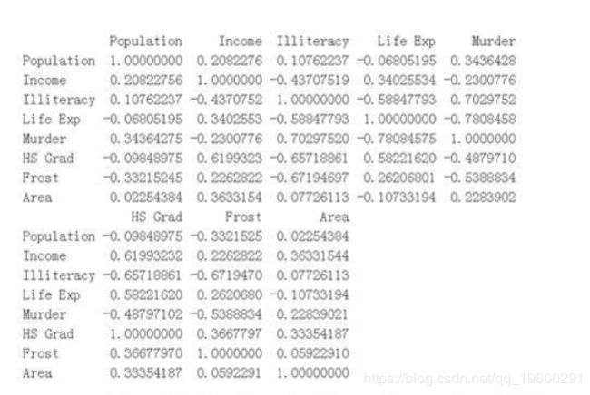
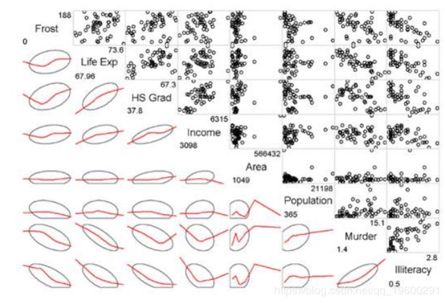
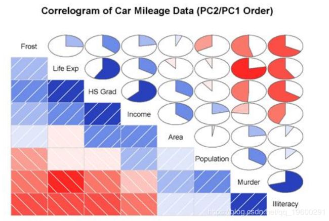
Murder histogram correlation analysis To see the relationships between the different variables, plot the scatter plot between the different variables`
Population Income Illiteracy Life Exp Murder
Population 1.00000000 0.2082276 0.10762237 -0.06805195 0.3436428
Income 0.20822756 1.0000000 -0.43707519 0.34025534 -0.2300776
Illiteracy 0.10762237 -0.4370752 1.00000000 -0.58847793 0.7029752
Life Exp -0.06805195 0.3402553 -0.58847793 1.00000000 -0.7808458
Murder 0.34364275 -0.2300776 0.70297520 -0.78084575 1.0000000
HS Grad -0.09848975 0.6199323 -0.65718861 0.58221620 -0.4879710
Frost -0.33215245 0.2262822 -0.67194697 0.26206801 -0.5388834
Area 0.02254384 0.3633154 0.07726113 -0.10733194 0.2283902
HS Grad Frost Area
Population -0.09848975 -0.3321525 0.02254384
Income 0.61993232 0.2262822 0.36331544
Illiteracy -0.65718861 -0.6719470 0.07726113
Life Exp 0.58221620 0.2620680 -0.10733194
Murder -0.48797102 -0.5388834 0.22839021
HS Grad 1.00000000 0.3667797 0.33354187
Frost 0.36677970 1.0000000 0.05922910
Area 0.33354187 0.0592291 1.00000000
`
From the plot,we can see murder has negative relationship with frost and life expectation.
Regression model regression model Regression model A mathematical model that quantitatively describes the statistical relationship. If the mathematical model of multivariate linear regression can be expressed as y = 0 + 1 * x + i, where 0, 1, ..., p are p + 1 parameters to be estimated, i are independent and obey the same normal distribution N (0, 2), y is a random variable; x can be a random variable or a non-random variable, i is called a regression coefficient, and the degree of influence of the independent variable on the dependent variable.``
Residuals:
Min 1Q Median 3Q Max
-3.4452 -1.1016 -0.0598 1.1758 3.2355
Coefficients:
Estimate Std. Error t value Pr(>|t|)
(Intercept) 1.222e+02 1.789e+01 6.831 2.54e-08 *
Population 1.880e-04 6.474e-05 2.905 0.00584 **
Income -1.592e-04 5.725e-04 -0.278 0.78232
Illiteracy 1.373e+00 8.322e-01 1.650 0.10641
Life Exp-1.655e+00 2.562e-01 -6.459 8.68e-08 *HS Grad3.234e-02 5.725e-02 0.565 0.57519Frost -1.288e-02 7.392e-03 -1.743 0.08867 .
Area 5.967e-06 3.801e-06 1.570 0.12391
---
Signif. codes: 0 '' 0.001 '' 0.01 '' 0.05 '.' 0.1 ' ' 1
Residual standard error: 1.746 on 42 degrees of freedom
Multiple R-squared: 0.8083, Adjusted R-squared: 0.7763
F-statistic: 25.29 on 7 and 42 DF, p-value: 3.872e-13
``
Perform a backward stepwise regression Then I use step regression to find optimal model``
Residuals:
Min 1Q Median 3Q Max
-3.2976 -1.0711 -0.1123 1.1092 3.4671
Coefficients:
Estimate Std. Error t value Pr(>|t|)
(Intercept) 1.202e+02 1.718e+01 6.994 1.17e-08 *
Population 1.780e-04 5.930e-05 3.001 0.00442 **
Illiteracy 1.173e+00 6.801e-01 1.725 0.09161 .
Life Exp-1.608e+00 2.324e-01 -6.919 1.50e-08 *Frost -1.373e-02 7.080e-03 -1.939 0.05888 .
Area 6.804e-06 2.919e-06 2.331 0.02439 *
---
Signif. codes: 0 '' 0.001 '' 0.01 '' 0.05 '.' 0.1 ' ' 1
Residual standard error: 1.712 on 44 degrees of freedom
Multiple R-squared: 0.8068, Adjusted R-squared: 0.7848
F-statistic: 36.74 on 5 and 44 DF, p-value: 1.221e-14
``
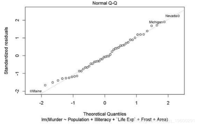
As can be seen from the output, the corresponding values are smaller than the significance level of 0.1, except for Density and region name, and the partial regression p number is significantly not zero at the significance level of 0.1. Note that the regression equation is significant. R-squared is about 0.8068 shows that the fitting effect of the equation is better. Significantly, we can see that Population , Life Exp, Area have a significant regression effect on murder. The residual analysis can test whether the stochastic error term is independent of the same distribution on the hypothesis of the regression model, and can also find the outlier. Fit and assess the chosen model for assumptions, outliers and influential observations The upper left graph is a scatter plot of the fitted and residuals. It can be seen from the graph that, except for the 6th outlier, all points are essentially randomly distributed in two ordinate values of -1 and +1 The lower left graph is the scatter plot of the standard deviation of the fitted and residual, and its meaning is similar to the above; the upper right graph shows that the random error term is subject to the normal distribution of the random error term, which means that the random error term has the same variance. , The reason is that the normal QQ diagram can be seen as a straight line; the lower right of the CooK distance map further confirmed that the sixth observation is an outlier, its impact on the regression equation is relatively large, according to specific Problem, discuss the actual background of this observation.conclusion From the results of the model, we can see the regression coefficients corresponding to each variable and his p-values. From the results of the model, it can be found that it has a smaller deviance. So the model can be considered better fit. Significantly, we can see that Population , Life Exp, Area have a significant regression effect on murder. Unfortunately, some of the variables are not significant, so in the subsequent analysis, we can reduce the data or feature variables selected processing, resulting in low latitude data, and try to get more significant variables.


