动手学深度学习PyTorch版——Task03学习笔记

过拟合、欠拟合及其解决方案

多项式函数拟合实验

%matplotlib inline
import torch
import numpy as np
import sys
sys.path.append("/home/kesci/input")
import d2lzh1981 as d2l
print(torch.__version__)

#初始化模型参数
n_train, n_test, true_w, true_b = 100, 100, [1.2, -3.4, 5.6], 5    #n_train是训练样本数，n_test是测试样本数
features = torch.randn((n_train + n_test, 1))
poly_features = torch.cat((features, torch.pow(features, 2), torch.pow(features, 3)), 1)    #poly_features是聚合特征
#features初始化为x，则poly_features初始化为x、x的平方，s的三次方
labels = (true_w[0] * poly_features[:, 0] + true_w[1] * poly_features[:, 1]
          + true_w[2] * poly_features[:, 2] + true_b)
labels += torch.tensor(np.random.normal(0, 0.01, size=labels.size()), dtype=torch.float)

features[:2], poly_features[:2], labels[:2]

#定义、训练和测试模型
def semilogy(x_vals, y_vals, x_label, y_label, x2_vals=None, y2_vals=None,
             legend=None, figsize=(3.5, 2.5)):    #定义一个绘图函数，用来观察训练误差和泛化误差的关系
    # d2l.set_figsize(figsize)
    d2l.plt.xlabel(x_label)
    d2l.plt.ylabel(y_label)
    d2l.plt.semilogy(x_vals, y_vals)
    if x2_vals and y2_vals:
        d2l.plt.semilogy(x2_vals, y2_vals, linestyle=':')
        d2l.plt.legend(legend)

num_epochs, loss = 100, torch.nn.MSELoss()

def fit_and_plot(train_features, test_features, train_labels, test_labels):   #这个函数用来训练模型，将训练误差和泛化误差打印出来，调用绘图函数
    # 初始化网络模型
    net = torch.nn.Linear(train_features.shape[-1], 1)
    # 通过Linear文档可知，pytorch已经将参数初始化了，所以我们这里就不手动初始化了
    
    # 设置批量大小
    batch_size = min(10, train_labels.shape[0])    
    dataset = torch.utils.data.TensorDataset(train_features, train_labels)      # 设置数据集
    train_iter = torch.utils.data.DataLoader(dataset, batch_size, shuffle=True) # 设置获取数据方式
    
    optimizer = torch.optim.SGD(net.parameters(), lr=0.01)                      # 设置优化函数，使用的是随机梯度下降优化
    train_ls, test_ls = [], []
    for _ in range(num_epochs):
        for X, y in train_iter:                                                 # 取一个批量的数据
            l = loss(net(X), y.view(-1, 1))                                     # 输入到网络中计算输出，并和标签比较求得损失函数
            optimizer.zero_grad()                                               # 梯度清零，防止梯度累加干扰优化
            l.backward()                                                        # 求梯度
            optimizer.step()                                                    # 迭代优化函数，进行参数优化
        train_labels = train_labels.view(-1, 1)
        test_labels = test_labels.view(-1, 1)
        train_ls.append(loss(net(train_features), train_labels).item())         # 将训练损失保存到train_ls中
        test_ls.append(loss(net(test_features), test_labels).item())            # 将测试损失保存到test_ls中
    print('final epoch: train loss', train_ls[-1], 'test loss', test_ls[-1])    
    semilogy(range(1, num_epochs + 1), train_ls, 'epochs', 'loss',
             range(1, num_epochs + 1), test_ls, ['train', 'test'])
    print('weight:', net.weight.data,
          '\nbias:', net.bias.data)

#三阶多项式函数拟合（正常）
fit_and_plot(poly_features[:n_train, :], poly_features[n_train:, :], labels[:n_train], labels[n_train:])

#线性函数拟合（欠拟合）
fit_and_plot(features[:n_train, :], features[n_train:, :], labels[:n_train], labels[n_train:])

#训练样本不足（过拟合）
fit_and_plot(poly_features[0:2, :], poly_features[n_train:, :], labels[0:2], labels[n_train:])

高维线性回归实验从零开始的实现

设维度p = 200，训练数据集样本数20

%matplotlib inline
import torch
import torch.nn as nn
import numpy as np
import sys
sys.path.append("/home/kesci/input")
import d2lzh1981 as d2l

print(torch.__version__)

#初始化模型参数
n_train, n_test, num_inputs = 20, 100, 200
true_w, true_b = torch.ones(num_inputs, 1) * 0.01, 0.05

features = torch.randn((n_train + n_test, num_inputs))
labels = torch.matmul(features, true_w) + true_b
labels += torch.tensor(np.random.normal(0, 0.01, size=labels.size()), dtype=torch.float)
train_features, test_features = features[:n_train, :], features[n_train:, :]
train_labels, test_labels = labels[:n_train], labels[n_train:]

# 定义参数初始化函数，初始化模型参数并且附上梯度
def init_params():
    w = torch.randn((num_inputs, 1), requires_grad=True)
    b = torch.zeros(1, requires_grad=True)
    return [w, b]

定义L2范数惩罚项
def l2_penalty(w):
    return (w**2).sum() / 2

定义训练和测试
batch_size, num_epochs, lr = 1, 100, 0.003
net, loss = d2l.linreg, d2l.squared_loss

dataset = torch.utils.data.TensorDataset(train_features, train_labels)
train_iter = torch.utils.data.DataLoader(dataset, batch_size, shuffle=True)

def fit_and_plot(lambd):   #重写fit_and_plot函数，传入超参数lambd，这个lambd是L2范数惩罚项最后要乘的整数
    w, b = init_params()
    train_ls, test_ls = [], []
    for _ in range(num_epochs):
        for X, y in train_iter:
            # 添加了L2范数惩罚项
            l = loss(net(X, w, b), y) + lambd * l2_penalty(w)
            l = l.sum()
            
            if w.grad is not None:
                w.grad.data.zero_()
                b.grad.data.zero_()
            l.backward()
            d2l.sgd([w, b], lr, batch_size)
        train_ls.append(loss(net(train_features, w, b), train_labels).mean().item())
        test_ls.append(loss(net(test_features, w, b), test_labels).mean().item())
    d2l.semilogy(range(1, num_epochs + 1), train_ls, 'epochs', 'loss',
                 range(1, num_epochs + 1), test_ls, ['train', 'test'])
    print('L2 norm of w:', w.norm().item())

观察过拟合
fit_and_plot(lambd=0)   #lambd=0表示不使用梯度衰减来训练

使用权重衰减
fit_and_plot(lambd=3)   #lambd=3

高维线性回归的简洁实现

def fit_and_plot_pytorch(wd):
    # 对权重参数衰减。权重名称一般是以weight结尾
    net = nn.Linear(num_inputs, 1)
    nn.init.normal_(net.weight, mean=0, std=1)    #使用init模块进行参数初始化
    nn.init.normal_(net.bias, mean=0, std=1)
    optimizer_w = torch.optim.SGD(params=[net.weight], lr=lr, weight_decay=wd) # 对权重参数衰减    使用optim里的随机梯度下降函数来优化，梯度衰减封装在SGD中了，weight_decay用来设置是否启用权重衰减
    optimizer_b = torch.optim.SGD(params=[net.bias], lr=lr)  # 不对偏差参数衰减
    
    train_ls, test_ls = [], []
    for _ in range(num_epochs):
        for X, y in train_iter:
            l = loss(net(X), y).mean()
            optimizer_w.zero_grad()
            optimizer_b.zero_grad()
            
            l.backward()
            
            # 对两个optimizer实例分别调用step函数，从而分别更新权重和偏差
            optimizer_w.step()
            optimizer_b.step()
        train_ls.append(loss(net(train_features), train_labels).mean().item())
        test_ls.append(loss(net(test_features), test_labels).mean().item())
    d2l.semilogy(range(1, num_epochs + 1), train_ls, 'epochs', 'loss',
                 range(1, num_epochs + 1), test_ls, ['train', 'test'])
    print('L2 norm of w:', net.weight.data.norm().item())

fit_and_plot_pytorch(0)   #不使用权重衰减，过拟合

fit_and_plot_pytorch(3)    #使用权重衰减

丢弃法从零开始

%matplotlib inline
import torch
import torch.nn as nn
import numpy as np
import sys
sys.path.append("/home/kesci/input")
import d2lzh1981 as d2l

print(torch.__version__)

def dropout(X, drop_prob):   #实现丢弃法的功能
    X = X.float()
    assert 0 <= drop_prob <= 1   #assert看丢弃率是多少，在0到1之间则继续，否则报错
    keep_prob = 1 - drop_prob
    # 这种情况下把全部元素都丢弃
    if keep_prob == 0:      #keep_prob是保存率，为0表示全部丢弃
        return torch.zeros_like(X)
    mask = (torch.rand(X.shape) < keep_prob).float()   #随机生成一个x形状的矩阵，若其每个位置上的元素小于保存率，则该位置为1，否则该位置为0，生成mask
    
    return mask * X / keep_prob    #mask中是1的位置保留，0的位置丢弃，除以keep_prob是做1-p的拉伸

X = torch.arange(16).view(2, 8)
dropout(X, 0)   #丢弃率为0时

dropout(X, 0.5)   #丢弃率为0.5时

dropout(X, 1.0)    #丢弃率为1时

# 参数的初始化
num_inputs, num_outputs, num_hiddens1, num_hiddens2 = 784, 10, 256, 256

W1 = torch.tensor(np.random.normal(0, 0.01, size=(num_inputs, num_hiddens1)), dtype=torch.float, requires_grad=True)
b1 = torch.zeros(num_hiddens1, requires_grad=True)
W2 = torch.tensor(np.random.normal(0, 0.01, size=(num_hiddens1, num_hiddens2)), dtype=torch.float, requires_grad=True)
b2 = torch.zeros(num_hiddens2, requires_grad=True)
W3 = torch.tensor(np.random.normal(0, 0.01, size=(num_hiddens2, num_outputs)), dtype=torch.float, requires_grad=True)
b3 = torch.zeros(num_outputs, requires_grad=True)

params = [W1, b1, W2, b2, W3, b3]

drop_prob1, drop_prob2 = 0.2, 0.5    #这里有两层隐藏层，所以用两个丢弃率

def net(X, is_training=True):   #参数is_training决定是否在训练
    X = X.view(-1, num_inputs)
    H1 = (torch.matmul(X, W1) + b1).relu()
    if is_training:  # 只在训练模型时使用丢弃法
        H1 = dropout(H1, drop_prob1)  # 在第一层全连接后添加丢弃层
    H2 = (torch.matmul(H1, W2) + b2).relu()
    if is_training:
        H2 = dropout(H2, drop_prob2)  # 在第二层全连接后添加丢弃层
    return torch.matmul(H2, W3) + b3

def evaluate_accuracy(data_iter, net):   #评估准确率时要判断是否使用了丢弃法
    acc_sum, n = 0.0, 0
    for X, y in data_iter:
        if isinstance(net, torch.nn.Module):
            net.eval() # 评估模式, 这会关闭dropout
            acc_sum += (net(X).argmax(dim=1) == y).float().sum().item()
            net.train() # 改回训练模式
        else: # 自定义的模型
            if('is_training' in net.__code__.co_varnames): # 如果有is_training这个参数
                # 将is_training设置成False
                acc_sum += (net(X, is_training=False).argmax(dim=1) == y).float().sum().item() 
            else:
                acc_sum += (net(X).argmax(dim=1) == y).float().sum().item() 
        n += y.shape[0]
    return acc_sum / n

#训练
num_epochs, lr, batch_size = 5, 100.0, 256  # 这里的学习率设置的很大，原因与之前相同。
loss = torch.nn.CrossEntropyLoss()
train_iter, test_iter = d2l.load_data_fashion_mnist(batch_size, root='/home/kesci/input/FashionMNIST2065')
d2l.train_ch3(
    net,
    train_iter,
    test_iter,
    loss,
    num_epochs,
    batch_size,
    params,
    lr)

丢弃法简洁实现

#神经网络的定义
net = nn.Sequential(
        d2l.FlattenLayer(),
        nn.Linear(num_inputs, num_hiddens1),
        nn.ReLU(),
        nn.Dropout(drop_prob1),
        nn.Linear(num_hiddens1, num_hiddens2), 
        nn.ReLU(),
        nn.Dropout(drop_prob2),
        nn.Linear(num_hiddens2, 10)
        )  
        '''
        FlattenLayer将图片转换成输入的格式
        Linear调用线性层，是隐藏层
        ReLU()激活
        Dropout丢弃法
        Linear第二层隐藏层
        Linear(num_hiddens2, 10)全连接输入层，将第二层隐藏层的输出输入
        '''

for param in net.parameters():   #将每个参数初始化
    nn.init.normal_(param, mean=0, std=0.01)

optimizer = torch.optim.SGD(net.parameters(), lr=0.5)
d2l.train_ch3(net, train_iter, test_iter, loss, num_epochs, batch_size, None, None, optimizer)

学习笔记

训练误差 ：模型在训练数据集上表现出的误差，
泛化误差 ： 模型在任意一个测试数据样本上表现出的误差的期望，常常用测试数据集上的误差来近似。
二者的计算都可使用损失函数（平方损失、交叉熵）
机器学习模型应关注降低泛化误差

模型选择：
验证数据集：训练数据集、测试数据集以外的一部分数据。简称验证集。因不可从训练误差估计泛化误差，无法依赖训练数据调参（选择模型）。
K折交叉验证：将原始训练数据集分割为K个不重合子数据集，之后做K次模型训练和验证。每次用一个子数据集验证模型，同时使用其他子数据集训练模型。最后将这K次训练误差以及验证误差各求平均数。
　　　　　　
欠拟合：模型不能得到较低的训练误差。
过拟合：模型的训练误差<<其在测试数据集上的误差
影响因素：有多种因素，而且实践中要尽力同时掌控欠拟合和过拟合。这有两个重要因素：模型复杂度、训练数据集大小。
模型复杂度：在模型过于简单时，泛化误差和训练误差都很高——欠拟合。在模型过于复杂时，训练误差有了明显降低，但泛化误差会越来越高——过拟合。所以我们需要一个最佳值。如图像。

训练数据集大小：训练数据集大小是影响着欠拟合和过拟合的一个重要因素。一般情况下，训练数据集中样本过少，会发生过拟合。但泛化误差不会随着训练数据集样本数的增加而增大。故在计算资源许可范围内，尽量将训练数据集调大一些。在模型复杂度较高（如：层数较多的深度学习模型）效果很好。

解决过拟合的方法有：权重衰减（L2范数正则化）、丢弃法
1.权重衰减：　　　
　　　　方法：正则化通过为模型的损失函数加入惩罚项，从而令得出的模型参数值较小。
　　　　权重衰减等价于L2范数正则化，经常用于应对过拟合现象。
　　　　L2范数正则化：
　　　　　　在模型原损失函数基础上添加L2范数惩罚项，从而的发哦训练所需最小化的函数。
　　　　　　　　L2范数惩罚项：模型权重参数每个元素的平方和与一个正的常数的乘积。
2.丢弃法：
　　　　方法：在隐藏层每个单元设置丢弃的概率，如：p。那么有 p 的单元的概率就会被清零，有1-p的概率的单元会被拉伸。
　　　　丢弃法不改变输入的期望值。
　　　　在测试模型时，为了拿到更加确定性的结果，一般不使用丢弃法。

梯度消失、梯度爆炸以及Kaggle房价预测

Kaggle 房价预测实战

%matplotlib inline
import torch
import torch.nn as nn
import numpy as np
import pandas as pd
import sys
sys.path.append("/home/kesci/input")
import d2lzh1981 as d2l
print(torch.__version__)
torch.set_default_tensor_type(torch.FloatTensor)

获取和读取数据集

test_data = pd.read_csv("/home/kesci/input/houseprices2807/house-prices-advanced-regression-techniques/test.csv")
train_data = pd.read_csv("/home/kesci/input/houseprices2807/house-prices-advanced-regression-techniques/train.csv")

train_data.shape

test_data.shape

train_data.iloc[0:4, [0, 1, 2, 3, -3, -2, -1]]

all_features = pd.concat((train_data.iloc[:, 1:-1], test_data.iloc[:, 1:]))

预处理数据

numeric_features = all_features.dtypes[all_features.dtypes != 'object'].index
all_features[numeric_features] = all_features[numeric_features].apply(
    lambda x: (x - x.mean()) / (x.std()))
# 标准化后，每个数值特征的均值变为0，所以可以直接用0来替换缺失值
all_features[numeric_features] = all_features[numeric_features].fillna(0)

# dummy_na=True将缺失值也当作合法的特征值并为其创建指示特征
all_features = pd.get_dummies(all_features, dummy_na=True)
all_features.shape

n_train = train_data.shape[0]
train_features = torch.tensor(all_features[:n_train].values, dtype=torch.float)
test_features = torch.tensor(all_features[n_train:].values, dtype=torch.float)
train_labels = torch.tensor(train_data.SalePrice.values, dtype=torch.float).view(-1, 1)

训练模型

loss = torch.nn.MSELoss()

def get_net(feature_num):
    net = nn.Linear(feature_num, 1)
    for param in net.parameters():
        nn.init.normal_(param, mean=0, std=0.01)
    return net

def log_rmse(net, features, labels):   #对数均方根误差来评价模型
    with torch.no_grad():
        # 将小于1的值设成1，使得取对数时数值更稳定
        clipped_preds = torch.max(net(features), torch.tensor(1.0))
        rmse = torch.sqrt(2 * loss(clipped_preds.log(), labels.log()).mean())
    return rmse.item()

def train(net, train_features, train_labels, test_features, test_labels,
          num_epochs, learning_rate, weight_decay, batch_size):
    train_ls, test_ls = [], []
    dataset = torch.utils.data.TensorDataset(train_features, train_labels)
    train_iter = torch.utils.data.DataLoader(dataset, batch_size, shuffle=True)
    # 这里使用了Adam优化算法
    optimizer = torch.optim.Adam(params=net.parameters(), lr=learning_rate, weight_decay=weight_decay) 
    net = net.float()
    for epoch in range(num_epochs):
        for X, y in train_iter:
            l = loss(net(X.float()), y.float())
            optimizer.zero_grad()
            l.backward()
            optimizer.step()
        train_ls.append(log_rmse(net, train_features, train_labels))
        if test_labels is not None:
            test_ls.append(log_rmse(net, test_features, test_labels))
    return train_ls, test_ls

K折交叉验证

def get_k_fold_data(k, i, X, y):    #用来选择模型设计并调节参数
    # 返回第i折交叉验证时所需要的训练和验证数据
    assert k > 1
    fold_size = X.shape[0] // k
    X_train, y_train = None, None
    for j in range(k):
        idx = slice(j * fold_size, (j + 1) * fold_size)
        X_part, y_part = X[idx, :], y[idx]
        if j == i:
            X_valid, y_valid = X_part, y_part
        elif X_train is None:
            X_train, y_train = X_part, y_part
        else:
            X_train = torch.cat((X_train, X_part), dim=0)
            y_train = torch.cat((y_train, y_part), dim=0)
    return X_train, y_train, X_valid, y_valid

def k_fold(k, X_train, y_train, num_epochs,
           learning_rate, weight_decay, batch_size):   #进行K折交叉验证，训练K次并返回每次训练和验证的平均误差
    train_l_sum, valid_l_sum = 0, 0
    for i in range(k):
        data = get_k_fold_data(k, i, X_train, y_train)
        net = get_net(X_train.shape[1])
        train_ls, valid_ls = train(net, *data, num_epochs, learning_rate,
                                   weight_decay, batch_size)
        train_l_sum += train_ls[-1]
        valid_l_sum += valid_ls[-1]
        if i == 0:
            d2l.semilogy(range(1, num_epochs + 1), train_ls, 'epochs', 'rmse',
                         range(1, num_epochs + 1), valid_ls,
                         ['train', 'valid'])
        print('fold %d, train rmse %f, valid rmse %f' % (i, train_ls[-1], valid_ls[-1]))
    return train_l_sum / k, valid_l_sum / k

模型选择

k, num_epochs, lr, weight_decay, batch_size = 5, 100, 5, 0, 64
train_l, valid_l = k_fold(k, train_features, train_labels, num_epochs, lr, weight_decay, batch_size)
print('%d-fold validation: avg train rmse %f, avg valid rmse %f' % (k, train_l, valid_l))

预测并在Kaggle中提交结果

def train_and_pred(train_features, test_features, train_labels, test_data,
                   num_epochs, lr, weight_decay, batch_size):
    net = get_net(train_features.shape[1])
    train_ls, _ = train(net, train_features, train_labels, None, None,
                        num_epochs, lr, weight_decay, batch_size)
    d2l.semilogy(range(1, num_epochs + 1), train_ls, 'epochs', 'rmse')
    print('train rmse %f' % train_ls[-1])
    preds = net(test_features).detach().numpy()
    test_data['SalePrice'] = pd.Series(preds.reshape(1, -1)[0])
    submission = pd.concat([test_data['Id'], test_data['SalePrice']], axis=1)
    submission.to_csv('./submission.csv', index=False)
    # sample_submission_data = pd.read_csv("../input/house-prices-advanced-regression-techniques/sample_submission.csv")

train_and_pred(train_features, test_features, train_labels, test_data, num_epochs, lr, weight_decay, batch_size)

学习笔记

梯度消失和梯度爆炸：
　　　　深度模型有关数值稳定性的典型问题是梯度消失和梯度爆炸。当神经网络的层数较多时，模型的数值稳定性更容易变差。
　　　　层数较多时，梯度的计算也容易出现消失或爆炸。
　　　　
随机初始化模型参数：
　　　　在神经网络中，需要随机初始化参数。因为，神经网络模型在层之间各个单元具有对称性。否则会出错。
　　　　若将每个隐藏单元参数都初始化为相等的值，则在正向传播时每个隐藏单元将根据相同的输入计算出相同的值，并传递至输出层。在反向传播中，每个隐藏单元的参数梯度相等。因此，这些参数在使用基于梯度的优化算法迭代后值依然相等。之后的迭代亦是如此。 据此，无论隐藏单元有几个，隐藏层本质上只有一个隐藏单元在发挥作用。所以，通常将神经网络的模型参数，进行随机初始化以避免上述问题。
　　　　PyTorch的默认随机初始化：
　　　 　PyTorch中，nn.Module的模块参数都采取了较合理的初始化策略，一般不用考虑。
　　　　Xavier随机初始化：
　　　　　　Xavier随机初始化将使用该全连接层中权重参数的每个元素都随机采样于均匀分布U。模型参数初始化后，每层输出的方差不受该层输入个数影响，且每层梯度方差也不受该层输出个数影响。
　　　　　　
考虑环境因素：
协变量偏移：
　　　设虽输入的分布可能随时间而变，但标记函数（条件分布P（y|x））不会改变。但在实践中容易忽视。例如用卡通图片作为训练集训练猫狗的识别分类。在一个看起来与测试集有着本质不同的数据集上进行训练，而不考虑如何适应新的情况，这很糟糕。这种协变量变化是因为问题的根源在于特征分布的变化（协变量的变化）。数学上可以说P（x)变了，但P（y|x) 保持不变。当认为x导致y时，协变量移位通常是正确假设。
标签偏移：
　　　导致标签偏移是标签P（y) 上的边缘分布的变化，但类条件分布是不变的P（x|y）是，会出现相反问题。当我们认为y导致x时，标签偏移是一个合理的假设。 病因（要预测的诊断结果）导致 症状（观察到的结果）。
　　　训练数据集，数据很少且只包含流感p（y）的样本。而测试数据集有流感p（y）和流感q（y），其中不变的时流感症状p（x|y）。这里就认为发生了标签的偏移。
概念偏移：
　　　相同的概念由于地理位置不同，标签本身的定义发生变化的情况。如果我们要建立一个机器翻译系统，分布P（y∣x）可能因我们的位置而异。这个问题很难发现。另一个可取之处是P（y∣x）通常只是逐渐变化。

循环神经网络的进阶

门控循环单元

载入数据集

import os
os.listdir('/home/kesci/input')

import numpy as np
import torch
from torch import nn, optim
import torch.nn.functional as F

import sys
sys.path.append("../input/")
import d2l_jay9460 as d2l
device = torch.device('cuda' if torch.cuda.is_available() else 'cpu')

(corpus_indices, char_to_idx, idx_to_char, vocab_size) = d2l.load_data_jay_lyrics()

初始化参数

num_inputs, num_hiddens, num_outputs = vocab_size, 256, vocab_size
print('will use', device)

def get_params():  
    def _one(shape):   #用来做权重的初始化，即Wxh和Whh的初始化
        ts = torch.tensor(np.random.normal(0, 0.01, size=shape), device=device, dtype=torch.float32) #随机正态分布初始化
        return torch.nn.Parameter(ts, requires_grad=True)
    def _three():
        return (_one((num_inputs, num_hiddens)),
                _one((num_hiddens, num_hiddens)),
                torch.nn.Parameter(torch.zeros(num_hiddens, device=device, dtype=torch.float32), requires_grad=True))
                #torch.zeros是全零初始化
     
    W_xz, W_hz, b_z = _three()  # 更新门参数
    W_xr, W_hr, b_r = _three()  # 重置门参数
    W_xh, W_hh, b_h = _three()  # 候选隐藏状态参数
    
    # 输出层参数
    W_hq = _one((num_hiddens, num_outputs))
    b_q = torch.nn.Parameter(torch.zeros(num_outputs, device=device, dtype=torch.float32), requires_grad=True)
    return nn.ParameterList([W_xz, W_hz, b_z, W_xr, W_hr, b_r, W_xh, W_hh, b_h, W_hq, b_q])

def init_gru_state(batch_size, num_hiddens, device):   #隐藏状态初始化
    return (torch.zeros((batch_size, num_hiddens), device=device), )

GRU模型（门控循环单元模型）

def gru(inputs, state, params):
    W_xz, W_hz, b_z, W_xr, W_hr, b_r, W_xh, W_hh, b_h, W_hq, b_q = params
    H, = state
    outputs = []
    for X in inputs:
        Z = torch.sigmoid(torch.matmul(X, W_xz) + torch.matmul(H, W_hz) + b_z)
        R = torch.sigmoid(torch.matmul(X, W_xr) + torch.matmul(H, W_hr) + b_r)
        H_tilda = torch.tanh(torch.matmul(X, W_xh) + R * torch.matmul(H, W_hh) + b_h)
        H = Z * H + (1 - Z) * H_tilda
        Y = torch.matmul(H, W_hq) + b_q
        outputs.append(Y)
    return outputs, (H,)

训练模型

num_epochs, num_steps, batch_size, lr, clipping_theta = 160, 35, 32, 1e2, 1e-2
pred_period, pred_len, prefixes = 40, 50, ['分开', '不分开']

d2l.train_and_predict_rnn(gru, get_params, init_gru_state, num_hiddens,
                          vocab_size, device, corpus_indices, idx_to_char,
                          char_to_idx, False, num_epochs, num_steps, lr,
                          clipping_theta, batch_size, pred_period, pred_len,
                          prefixes)

门控循环单元的pytorch实现

不需要初始化参数，也不需要自己写GRU，只需调用nn.GRU

num_hiddens=256
num_epochs, num_steps, batch_size, lr, clipping_theta = 160, 35, 32, 1e2, 1e-2
pred_period, pred_len, prefixes = 40, 50, ['分开', '不分开']

lr = 1e-2 # 注意调整学习率
gru_layer = nn.GRU(input_size=vocab_size, hidden_size=num_hiddens)
model = d2l.RNNModel(gru_layer, vocab_size).to(device)
d2l.train_and_predict_rnn_pytorch(model, num_hiddens, vocab_size, device,
                                corpus_indices, idx_to_char, char_to_idx,
                                num_epochs, num_steps, lr, clipping_theta,
                                batch_size, pred_period, pred_len, prefixes)

LSTM（长短期记忆）

import numpy as np
import torch
from torch import nn, optim
import torch.nn.function as F

import sys
sys.path.append("../input/")
import d2lzhpytorch as d2l
device = torch.device('CUDA' if torch.cuda.is_available() else 'CPU')

(corpus_indices, char_to_idx, idx_to_char, vocab_size) = d2l.load_data_jay_lyrics()

初始化参数

num_inputs, num_hiddens, num_outputs = vocab_size, 256, vocab_size
print('will use', device)

def get_params():
    def _one(shape):
        ts = torch.tensor(np.random.normal(0, 0.01, size=shape), device=device, dtype=torch.float32)
        return torch.nn.Parameter(ts, requires_grad=True)
    def _three():
        return (_one((num_inputs, num_hiddens)),
                _one((num_hiddens, num_hiddens)),
                torch.nn.Parameter(torch.zeros(num_hiddens, device=device, dtype=torch.float32), requires_grad=True))
    
    W_xi, W_hi, b_i = _three()  # 输入门参数
    W_xf, W_hf, b_f = _three()  # 遗忘门参数
    W_xo, W_ho, b_o = _three()  # 输出门参数
    W_xc, W_hc, b_c = _three()  # 候选记忆细胞参数
    
    # 输出层参数
    W_hq = _one((num_hiddens, num_outputs))
    b_q = torch.nn.Parameter(torch.zeros(num_outputs, device=device, dtype=torch.float32), requires_grad=True)
    return nn.ParameterList([W_xi, W_hi, b_i, W_xf, W_hf, b_f, W_xo, W_ho, b_o, W_xc, W_hc, b_c, W_hq, b_q])

def init_lstm_state(batch_size, num_hiddens, device):
    return (torch.zeros((batch_size, num_hiddens), device=device), 
            torch.zeros((batch_size, num_hiddens), device=device))

LSTM模型

def lstm(inputs, state, params):
    [W_xi, W_hi, b_i, W_xf, W_hf, b_f, W_xo, W_ho, b_o, W_xc, W_hc, b_c, W_hq, b_q] = params
    (H, C) = state
    outputs = []
    for X in inputs:
        I = torch.sigmoid(torch.matmul(X, W_xi) + torch.matmul(H, W_hi) + b_i)
        F = torch.sigmoid(torch.matmul(X, W_xf) + torch.matmul(H, W_hf) + b_f)
        O = torch.sigmoid(torch.matmul(X, W_xo) + torch.matmul(H, W_ho) + b_o)
        C_tilda = torch.tanh(torch.matmul(X, W_xc) + torch.matmul(H, W_hc) + b_c)
        C = F * C + I * C_tilda
        H = O * C.tanh()
        Y = torch.matmul(H, W_hq) + b_q
        outputs.append(Y)
    return outputs, (H, C)

训练模型

num_epochs, num_steps, batch_size, lr, clipping_theta = 160, 35, 32, 1e2, 1e-2
pred_period, pred_len, prefixes = 40, 50, ['分开', '不分开']

d2l.train_and_predict_rnn(lstm, get_params, init_lstm_state, num_hiddens,
                          vocab_size, device, corpus_indices, idx_to_char,
                          char_to_idx, False, num_epochs, num_steps, lr,
                          clipping_theta, batch_size, pred_period, pred_len,
                          prefixes)

LSTM的pytorch实现

num_epochs, num_steps, batch_size, lr, clipping_theta = 160, 35, 32, 1e2, 1e-2
pred_period, pred_len, prefixes = 40, 50, ['分开', '不分开']

lr = 1e-2 # 注意调整学习率
lstm_layer = nn.LSTM(input_size=vocab_size, hidden_size=num_hiddens)
model = d2l.RNNModel(lstm_layer, vocab_size)
d2l.train_and_predict_rnn_pytorch(model, num_hiddens, vocab_size, device,
                                corpus_indices, idx_to_char, char_to_idx,
                                num_epochs, num_steps, lr, clipping_theta,
                                batch_size, pred_period, pred_len, prefixes)

深度循环神经网络

import numpy as np
import torch
from torch import nn, optim
import torch.nn.function as F

import sys
sys.path.append("../input/")
import d2lzhpytorch as d2l
device = torch.device('CUDA' if torch.cuda.is_available() else 'CPU')

(corpus_indices, char_to_idx, idx_to_char, vocab_size) = d2l.load_data_jay_lyrics()

num_hiddens=256
num_epochs, num_steps, batch_size, lr, clipping_theta = 160, 35, 32, 1e2, 1e-2
pred_period, pred_len, prefixes = 40, 50, ['分开', '不分开']

lr = 1e-2 # 注意调整学习率

gru_layer = nn.LSTM(input_size=vocab_size, hidden_size=num_hiddens,num_layers=2)   #num_layers=2表示两层循环神经网络
model = d2l.RNNModel(gru_layer, vocab_size).to(device)
d2l.train_and_predict_rnn_pytorch(model, num_hiddens, vocab_size, device,
                                corpus_indices, idx_to_char, char_to_idx,
                                num_epochs, num_steps, lr, clipping_theta,
                                batch_size, pred_period, pred_len, prefixes)

gru_layer = nn.LSTM(input_size=vocab_size, hidden_size=num_hiddens,num_layers=6)
model = d2l.RNNModel(gru_layer, vocab_size).to(device)
d2l.train_and_predict_rnn_pytorch(model, num_hiddens, vocab_size, device,
                                corpus_indices, idx_to_char, char_to_idx,
                                num_epochs, num_steps, lr, clipping_theta,
                                batch_size, pred_period, pred_len, prefixes)

双向循环神经网络

import numpy as np
import torch
from torch import nn, optim
import torch.nn.function as F

import sys
sys.path.append("../input/")
import d2lzhpytorch as d2l
device = torch.device('CUDA' if torch.cuda.is_available() else 'CPU')

(corpus_indices, char_to_idx, idx_to_char, vocab_size) = d2l.load_data_jay_lyrics()

num_hiddens=128
num_epochs, num_steps, batch_size, lr, clipping_theta = 160, 35, 32, 1e-2, 1e-2
pred_period, pred_len, prefixes = 40, 50, ['分开', '不分开']

lr = 1e-2 # 注意调整学习率

gru_layer = nn.GRU(input_size=vocab_size, hidden_size=num_hiddens,bidirectional=True)  #bidirectional=True表示使用双向循环神经网络
model = d2l.RNNModel(gru_layer, vocab_size).to(device)
d2l.train_and_predict_rnn_pytorch(model, num_hiddens, vocab_size, device,
                                corpus_indices, idx_to_char, char_to_idx,
                                num_epochs, num_steps, lr, clipping_theta,
                                batch_size, pred_period, pred_len, prefixes)

学习笔记

1.门控循环神经网络：捕捉时间序列中时间步距离较⼤的依赖关系，通过学习的门控制信息的流动，用于解决梯度衰减问题
常用的门控神经网络有：GRU(门控循环单元)和LSTM(长短期记忆)
（1）GRU

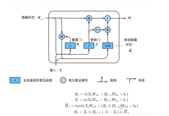
重置⻔：有助于捕捉时间序列⾥短期的依赖关系；
更新⻔：有助于捕捉时间序列⾥⻓期的依赖关系。
（2）LSTM

遗忘门:控制上一时间步的记忆细胞 输入门:控制当前时间步的输入
输出门:控制从记忆细胞到隐藏状态
记忆细胞：⼀种特殊的隐藏状态的信息的流动
2.深度循环神经网络

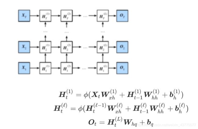
深度循环神经网络不是越深越好，越深对于数据集要求更高。
3.双向循环神经网络

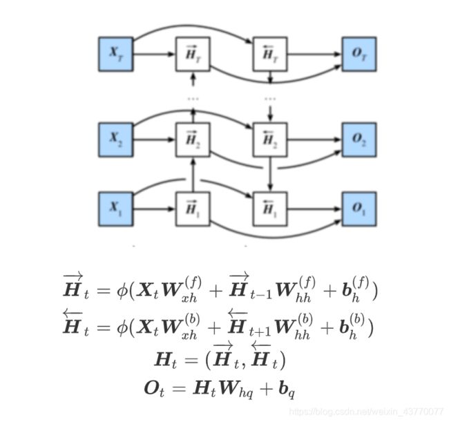
双向循环神经网络中两者隐藏状态H的连接是1维连接，也就是concat中参数dim=1，最后1维的维度变为两者1维维度之和