【DL by Ng】Deeplearning.ai 深度学习工程师课程 -- By Andrew Ng 吴恩达

三个版本

• deeplearning.ai 付费版本, 带练习.
• Coursera 版本
• 网易云课堂翻译版本, 练习题需要自己找. 但是网速快, 可以下载观看.

这里笔记用的是网易云课堂的版本.

I. 神经网络和深度学习

Week 01. 深度学习概论 Introduction

Lecture 001 ： 欢迎来到深度学习工程师微专业

喜欢 Ng 普通话的声音

我希望可以培养成千上万的人使用人工智能, 去解决真实世界的实际问题, 创造一个人工智能驱动的社会.

Lecture 002 : 什么是神经网络?

以 housing Price Prediction 为例, 讲解了构成 神经网络的三个基本要素

• input layer : initial features, X
• hidden layers : high-level features, some could be explained, most couldn’t\
• output layer : Y

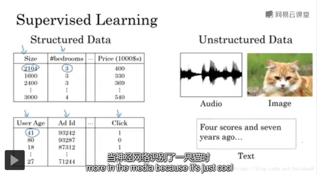
Lecture 003 : Supervised Learning with Neural Networks

• some common tasks of Supervised Learning using specific NNs

Possibly the single most lucrative application of deep learning today is online advertising. maybe not the most inspiring, but certainly very lucrative.

• Structured data VS Unstructured data
  

Lecture 004 : Why is deep learning taking off?

• Scale drives deep learning progress
  • scale of data, digital labeled data
  • scale of NNs, lots of inputs, hidden layers, connections …

Lecture 004: About this Course

Lecture 005: Course Resources

forum, e-mails, etc

Week 02: Basics of Neural Network programming

Lecture 001: Binary Classification

Lecture 002: Logistic Regression

• Logistic Regression : 在 linear regression 的外面套上 sigmoid 函数.
  

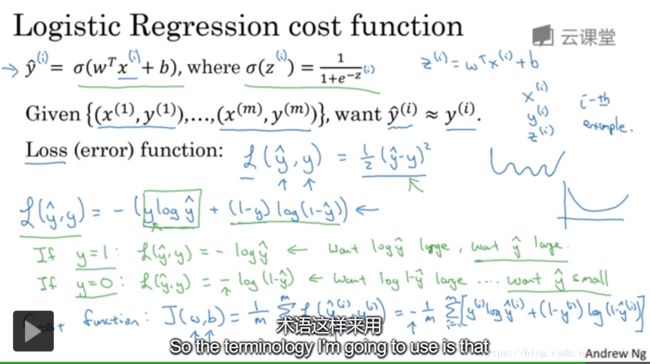
Lecture 003: Logistic Regression cost function

• Loss(error) function : on a single train example. Not using MSE, it’s not convex and hard to find optimal point using Gradient descent. So we need to design a convex one, taking advantages of $\hat{y}$ features.
• Cost function : measure the perfomance of $(\omega ,b)$on the full train set
  

Lecture 004: Gradient Descent

Lecture 005: Derivatives

Lecture 006: More derivative examples

Lecture 007: Computation Graph

• Left to Right : blue lines, forward-propagation
• Right to Left : red lines, back-propagation
  

Lecture 008: Derivatives with a Computation Graph

• back-propagation, calculate derivatives, chain rule

Lecture 009: Logistic regression derivatives

• input : $X=(x_1,x_2)$
• initial params : $w=(w_1,w_2),b$
• hidden layer: $z=w_1{x}_1+w_2{x}_2+b$
• activation function $a=\sigma (z)=\frac{1}{1+e^{-z}}$
• loss function $\mathcal{L}(a,y)=-(y\ln (a)+(1-y)\ln (1-a))$

calculation of derivatives

• $da=\frac{d\mathcal{L}(a,y)}{da}=-(\frac{y}{a}-\frac{1-y}{1-a})=-\frac{y}{a}+\frac{1-y}{1-a}$
• $dz=\frac{d\mathcal{L}}{da}\cdot \frac{da}{dz}=(-\frac{y}{a}+\frac{1-y}{1-a})\cdot a(1-a)=-y(1-a)+a(1-y)=a-y$
• $d{w}_1=(a-y)x_1$
• $d{w}_2=(a-y)x_2$
• $db=(a-y)$

so, in the next gradient descent phrase

$w_1:=w_1-\alpha d{w}_1$
$w_2:=w_2-\alpha d{w}_2$
$b:=b-\alpha db$

Lecture 010: Logistic regression on m examples

上一讲说的是 single examples 的栗子，对于有$m$个examples 的情况下，采用累加求平均的方式计算$dw，db$。
这里面计算最大的问题就是两层for-loop，外层是 m 个examples，内层是 n 个weights，复杂度是 $O(mn)$. 对于 DL 来说，这个值会非常大，下一讲来看如何使用向量化 vectorizazion 来摆脱for循环，加速计算。

Lecture 011: Vectorization

• vectorization 用来代替 explicit for-loops，达到加速目的
• 对于1M 数据， np.dot() 约 1.5ms，for-loop 约 500ms
• np.dot()这类的向量化处理，是利用SIMD(single instruction multiple data )技术，在 CPU／GPU 上均可以达到很良好的效果，GPU is better。

Lecture 012: More vectorization examples

• NN programming guideline : Whenever possible, avoid explicit for-loops.
  • Whenever thinking of using for-loops, find alternative vectorization solution in numpy.

Lecture 013: Vectorizing Logistic Regression

I’m super excited about this techinique, and when we talk about neural networks later, without using even a single explicit for loop.

• $Z=np.dot(w.T,X)+b$, where $b$ is a scalar and broadcasting to a vector$[b...b{]}_{1\times m}$

Lecture 014: Vectorizing Logistic Regression Gradient Descent

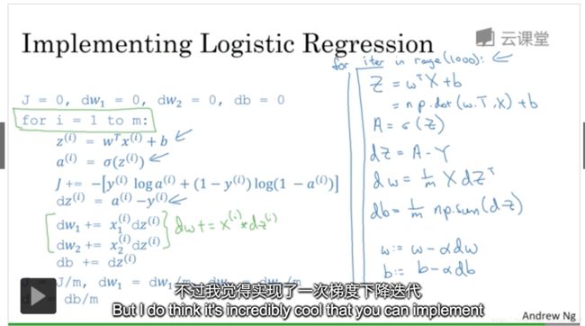
• propagation 和 back-propagation 全部实现了 vectorization
• 最外层的gradient descent 迭代次数，还是要用一层 explicit for-loop，这个没办法去掉

Lecture 015: Broadcasting in Python

一个栗子

import numpy as np

A = np.array([ [1,2,3,4],
			   [5,6,7,8],
			   [9,10,11,12] ])
sum_cols = A.sum(axis = 0)
percentage = A / sum_cols.reshape(1,4)

• A.sum() 默认对所有元素求和，返回一个scalar。参数 axis = 0 代表每列求和，返回一个 1x4 的 vector， axis = 1 代表每行求和，返回一个 3x1 的vector
• sum_cols 的reshape(1,4) 是多此一举，但是可以清晰的反应其shape，防止出错。reshape 的时间复杂度是 $O(1)$，所以不用担心性能损耗
• broadcasting 就是将 sum_cols 复制3层，变成和 A 相同的shape，然后进行 element-wise operations。

Lecture 016: A note on Python/Numpy vectors

a = np.random.randn(5) # a.shape = (5,), a bizarre `rank 1 array`, not a vector

a = np.random.randn(1,5) # a.shape = (1,5), good 

a = np.random.randn(5,1) # a.shape = (5,1), good

assert(a.shape == (1,5)) # check whether its shape suits what we expected

Lecture 017: Quick tour of Jupyter/ipython notebooks

Lecture 018: Explanation of logistic regression cost function(optional)

• The Loss function
  • $\hat{y}=\sigma (w^{T}x+b)$
  • we interpret $\hat{y}$ as $\hat{y}=p(y=1|x)$,
  • so, if $y=1,p(y|x)=\hat{y}$, if $y=0,p(y|x)=1-\hat{y}$
  • combine two to one $p(y|x)={\hat{y}}^y(1-\hat{y}{)}^{1-y}$
  • because the log function is a strictly monotonically increasing function, so maximize/minimize $p(y|x)$ equals to maximize/minimize $\log p(y|x)$ equals to max/min $\log {\hat{y}}^y(1-\hat{y}{)}^{1-y}=y\log \hat{y}+(1-y)\log (1-\hat{y})$
  • minimizing the loss ( $1-p(y|x)$ ) corresponding to maximizing the log of the probability, corresponding to minimizing the negative probability

Week 03: One hidden layer Neural Networks

Lecture 001: Neural Networks Overview

• multi-layer, $a_i^{[k]}$ the i-th node of k-th layer.
• each unit, is a combination of linear unit + activation function

Lecture 002: Neural Network Representation

• input layer, hidden layer, output layer
• But this is a 2 layers NN, the input layer is not counted, just for conversion.
  

Lecture 003: Computing a NN’s Output

what you see is that is like logistic regression but repeat of all the times.

Lecture 004: Vectorizing across multiple examples

• each column representes an example
• each row representes a hidden unit

Lecture 005: Explanation for vectorized implementation

Lecture 006: Activation Functions

• sigmoid $\sigma (z)=\frac{1}{1+e^{-z}}$, never use this except for output layer $(0,1)$
• tanh, $tanh(z)=\frac{e^z-e^{-z}}{e^z+e^{-z}}$, always better than sigmoid but worse than ReLU
• ReLU $ReLU(z)=\max (0,z)$, best , fast, most used.
• leaky ReLU $a=\max (0.01z,z)$

Lecture 007: Why do you need non-linear activation function?

It turns out that if you use a linear activation function, or alternatively if you don’t have an activation function, then no matter how many layers your neural network has, your NN always doing is just computing one single linear activation function, so you might as well not have any hidden layers.
Because the composition of two linear functions is itself a linear function, so unless you throw a non-linearity in there, then you’re not computing more interesting functions, even as you go deeper in the work.

Lecture 008: Derivatives of activation functions

• sigmoid function, $g(z)=\frac{1}{1+e^{-z}}\to g^{\prime }(z)=g(z)(1-g(z))$
• $tanh(z)=\frac{e^z-e^{-z}}{e^z+e^{-z}}\to tan{h}^{\prime }(z)=1-(tanh(z){)}^2$

Lecture 009: Gradient descent for neural networks

• forward propagation & back propagation
  

Lecture 010: Back-propagation intuition (Optional)

Lecture 011: Random Initialization

• What happens if you initialize weights to zero?

Because all the hidden units start off computing the same function, and both hidden units have the same influence on the output unit, No matter how long you train your neural network, all the hidden units are still computing exactly the same function. and so in this case, there is really no point to having more than one hidden unit.
The solution to this is to initalize your parameters randomly.

• we intend to initialize weights as a very small number to accelerate gradient descent.

Week 04: Deep Neural Networks

Lecture 001. Deep L-layer Neural Network

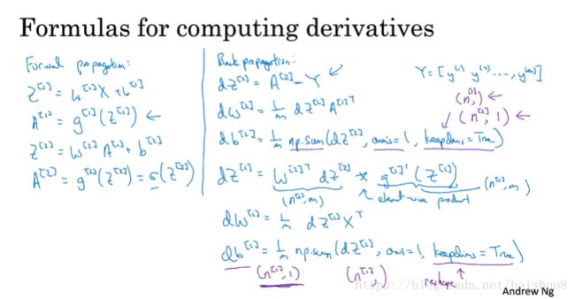
Lecture 002: Forward Propagation in a Deep Network

It turns out that we implement deep neural network, one of the ways to increase your odds of having bug-free implementation is to think very systematically and carefully about the matrix dimensions you’re working with. so when i’m trying to debug my own code I’ll often pull a piece of paper and just think carefully through the dimensions of the matrix I’m working with

Lecture 003: Getting your matrix dimensions right

Lecture 004: Why deep representations?

Some people like to make an analogy between deep neural networks and the human brain where we believe um… neuroscientists believe that the human brain also starts off detecting simple things like edges in what your eyes see and it builds those up to detect more complex things, like the faces that you see. I think analogies between deep learning and the human brain are sometimes a little bit dangerous. but you know there is a lot of truth, to this being how we think the human brain works and that the human brain probably detects simple things like edges first and put them togeter to form more and more complex objects. and so that has served as a loose form of inspiration for some deep learning as well.

Lecture 005: Building blocks of deep neural networks

• implementation tricks: cache $z^{[l]}$, and $w^{[l]}$, $b^{[l]}$

Lecture 006: Forward and Backward Propagation

• 存疑， $a^l=g^l(z^l)\to d{z}^l=d{a}^l÷g^l{}^{\prime }(z^l)$ ???
• 上述疑虑错误, 因为 notation 中 $d{z}^l$ 指的是从源头算起, $\frac{dJ}{d{z}^l}=\frac{dJ}{d{a}^l}\cdot \frac{d{a}^l}{d{z}^l}=d{a}^l\cdot g^l{}^{\prime }(z^l)$

Lecture 007: Parameters VS Hyperparameters

• Parameters: $w,b$

• Hyperparameters

  • learning rate $\alpha$
  • #iterations

  • hidden layers $L$

  • hidden units $n^1,n^2,...,n^L$

  • choice of activation function
  • momentum
  • mini-batch size
  • various forms of regularization parameters

• why we call them hyper-parameters? because they determine the real parameters.

• empirical process: try, try, try until find it

Lecture 008: What does this have to do with the brain?

II. 改善神经网络:超参数调参,正则化以及优化

Week 01: Setting up your ML application

Lecture 001: Train/dev/test sets

In this week, you’ll learn the practical aspects of how to make your neural network work well, ranging from things like hyper-parameter tuning to how to set up your data to how to make sure your optimization algorithm runs quickly.

And what I’ve seen is that intuitions from one domain or from one application area often do not transfer to other application areas. And the best choices may depend on the amount of data you have,

Cycle of Idea -> Code -> Experiment -> Idea -> Code -> Experiment

Train / Development / Test sets

• Train for train

• dev: for hold-out cross-validation

• Test

• In classical ML era, 70% / 30% , or 60%/20%/20%

• In modern big data era, a million examples in total, 10k is enough for dev/test. 98%/1%/1%

it’s OK to have no test set, only the result is biased estimation.

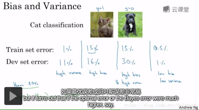
Lecture 002: Bias / Variance

I’ve noticed that almost all the really good machine learning practitioners tend to be very sophisticated in understanding of Bias and Variance. Bias and Variance is one of those concepts that’s easily learned but difficult to master. Even if you think you’ve seen the basic concepts of Bias and Variance, there’s often more new ones to it than you’d expect.
In DL trend, there’s less discussion about Bias-Variance trade-off.

The two key numbers to look at to understand bias and variance will be the train set error and the dev set error.

Lecture 003: Basic “Recipe” for ML

Lecture 004: Regularization

If you use L1 regularization, the w will end up being sparse, which means that the w vector will have lots of zeros in it. And some people say that this can help with compressing the model, although, I find that, in practice, L1 regularization to make your model sparse helps only a little bit. So I don’t think it’s used that much, at least not for the purpose of compressing your model.
L2 regularization is just used much much more often.
lambda is a key-word in Python, while writing Python code, use lambd for $\lambda$

• L2 norm regularization is also called weight decay, $d{w}^l=(\text{from backprop})+\frac{\lambda }{m}{w}^l\to w^l:=w^l-\alpha d{w}^l$

Lecture 005: Why regularization reduces overfitting?

• L2 regularization makes some weights decay to zero, so a trend from overfitting to underfitting, then there a midll value of $\lambda$ that makes the result just right.
  

• while using L2 normalization, $z$ is constraint to a small value near $0$, falls into the linearly part of activation function. so, the NN won’t be over sophisticated.

Lecture 006: Dropout regularization

• Dropout some hidde units randomly by zero them out to get a much dimimished network.
  

• Implementation of Inverted dropout

# illustrate with layer l = 3

# the prob of a unit being kept, (1-prob): the prob of a unit being dropped out
keep_prob = 0.8

# stands for keep-dropout distruibution
d3 = np.random.rand(a3.shape[0], a3.shape[1]) < keep_prob
# the dropped out ones are set to 0
a3 = np.multiply(a3, d3)
# invert the expectation of a3 to the origin full NN
a3 /= keep_prob

Lecture 007: Understanding dropout

• Intuition: Can’t rely on any one feature, so have to spread out weights.
• Dropout is mostly used in computer vision, almost as default. cause always not enough image data, CV always has a trend to over-fitting.
• while using dropout, you lose the well defined cost function $J$ and it becomes hard to calculate. so what I usually do is turn off dropout, and run my code and make sure that it is monotonically decreasing J. and the turn on dropout and hope that I didn’ introduce bugs into my code during dropout.

Lecture 008: Other regularization methods

• Data augmentation
  • flip horizentally
  • random crops of the image
• Early stopping

I personly prefer L2 normalization, and some differert values of $\lambda$

Lecture 009: Normalizing inputs

• Normalization steps

  1. subtract mean : $\mu =\frac{1}{m}\sum x^i,x:=x-\mu$
  2. normalize variance: ${\sigma }^2=\frac{1}{m}\sum (x^i{)}^2,x/={\sigma }^2$
  3. normalize your train set and test set

• Why normalize inputs?
  

010: Vanishing/Exploding gradients 梯度消失/梯度爆炸

• explode/vanish expotentially

• while using ReLU, $\text{w = np.sqrt}(\frac{2}{n^{[l-1]}})$

• while using tanh, use Xavier initialization $\text{w = np.sqrt}(\frac{1}{n^{[l-1]}})$

011: Weight initialization for DL

Hopefully that makes your weights, not explode too quickly and not decay to zero too quickly, so you can train a reasonably deep network without the weights or the gradiets exploding or vanishing too much.

012: Numerical approximation of gradients 梯度的数值逼近

• Two-sided difference formula is much more accurate than one-sided difference
  $$f^{\prime }(\theta )=\underset{ϵ\to 0}{\lim }\frac{f(\theta +ϵ)-f(\theta -ϵ)}{2ϵ}$$

013: Gradient Checking

Gradient checking is a technique that’s helped me save tons of time, and helped me find bugs in my implementations of back propagation many times.

014: Gradient Checking implementation notes

• Don’t use in training, – only to debug
• If algo fails grad check, look at components to try to identify bug
• Remember regularization
• Doesn’t work with dropout

Week 02: Optimization Algorithms

Lecture 001: Mini-batch gradient descent

Lecture 002: Understanding mini-batch gradient descent

Lecture 003: Exponentially weighted averages

Lecture 004: Understanding Exponentially weighted average

• Why called exp weighted average?

Lecture 005: Bias correction in exponentially weighted average

Bias correction can make your computation of these averages more accurately. Warm up.

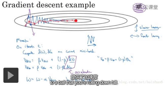
Lecture 006: Gradient descent with momentum

Gradient descent with momentum almost always works faster than
the standard gradient descent algorithm. In one sentence, the basic idea is to compute an exponentially weighted average of your gradients and then use that gradient to update your weights instead.

Lecture 007: RMSprop

• RMSprop, root mean square prop

Lecture 008: Adam optimization algorithm

• Adam: Adaptive Moment Estimation,

• Hyperparameters default values
  

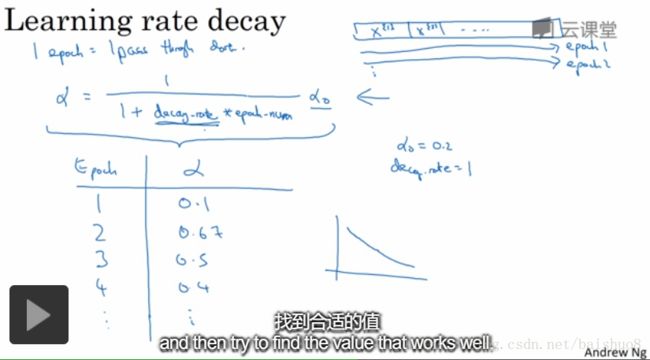
Lecture 008: Learning rate decay

Lecture 010: The problem of local optima

Week 03: Hyperparameter tuning & Batch Norm & Programming frameworks

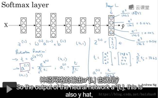
Lecture 008: Softmax regression

• C = #classes = 4 (0,1,2,…, C-1 )

• $n^{[}L]=4=C$, we want the probability to each class

• $\hat{y}size(4,1)$, contains 4 probabilities, sum to 1
  

• how to calculate it?
  

• softmax examples with no hidden layers, just produce linear boundaries

Lecture 009: Training a softmax classifier

• The name softmax contrast to hardmax

• Softmax regression generalizes logistic regression to C classes.

• if C=2, softmax regression regressioned to logistic regression.(only compute C0, Cother = 1 - C0)
  

• single loss function $L(\hat{y},y)=-{\sum }_{j=1}^n{y}_j\log \widehat{y_j}$

• total cost function $J(w,b)=\frac{1}{m}{\sum }_{i=1}^m{L}_i$
  

• The inital GD, $d{z}^{[L]}=\hat{y}-y$, a vector of size Cx1
  

Lecture 010: DL frameworks

Lecture 011: TensorFlow

• Basic version

import numpy as np
import tensorflow as tf

w = tf.Variable(0, dtype = tf.float32)
cost = tf.add(tf.add(w**2, tf.multiply(-10, w)), 25)
# same as
# cost = w**2 - 10*w + 25
train = tf.train.GradientDescentOptimizer(0.01).minimize(cost)

init = tf.global_variables_initializer()
session = tf.Session()
session.run(init)

//before gradient descent optimization
print(session.run(w)) # 0.0
//run optimization
session.run(train)
print(session.run(w)) # 0.1
// run 1000 times
for i in range(1000):
	session.run(train)
print(session.run(w)) # 4.99999

• Importing train data set as parameters

import numpy as np
import tensorflow as tf

coefficients = np.array([ [1], [-20], [25] ])

w = tf.Variable([0], dtype=tf.float32)
x = tf.placeholder(tf.float32, [3,1])
cost = x[0][0]*w**2 + x[1][0]*w + x[2][0]
train = tf.train.GradientDescentOptimizer(0.01).minimize(cost)
init = tf.global_variables_initializer()

with tf.Session() as session:
	session.run(init)
	for i in range(1000):
		session.run(train, feed_dict = {x:coefficients} )
	print(seesion.run(w))

III. 结构化机器学习项目

IV. 卷积神经网络 CNN

Week 01: CNN

Lecture 001: Computer Vision

• Image classification: A cat or not?
• Object detection: Find the cars and locate them
• Neural Style Transfer: CNN artist
• If we use the raw image, there will be too big featuremaps, for example, an RGB image of size 1000 x 1000, the feature number is 3M. if we have 1k hidden units in layer1, we’ll have 3 billion parameters to fit. Impossible work! -> That’s why we inrouduce convolutional operations.

Lecture 002: Edge detection example

Lecture 003: More edge detections

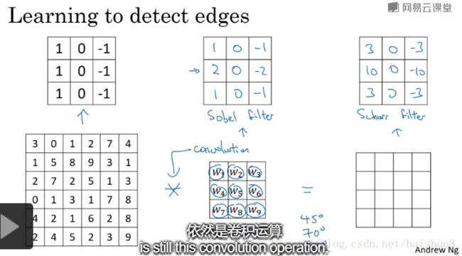
So the idea that you can treat these 9 numbers as parameters, to be learned, has been one ot the most powerful ideas in computer vision.

Lecture 004: Padding

Let’s say, an image of size$n\times n$, a filter of size $f\times f$, so the size of output is

• No padding : 从左向右滑动, 每一列都做一个filter, 但是最后 $f-1$列没有filter 了, so 最后的size : $(n - (f-1)) \times (n - (f-1)) $

  • But the size of original image is shrinked,
  • and the edge corner pixels was visited much less than central pixels, thus lots of edge information is lost

• Padding to preserve the original size, the missing size of each direction is $(f-1)$, and we padding two sides of that direction, so the padding size is $ p = \frac {(f-1)}{2}$, the original image is padded to size $(n+2p)\times (n+2p)$, if we only know $n,p,f$, the output size is $(n+2p-(f-1))\times (n+2p-(f-1))$, particularly, if $ p = \frac {(f-1)}{2}$, the output size is $n \times n $

• terminology : valid or same convolutions

  • valid: no padding, all pixels are valid real-value, $$n\times n\ast f\times f\to (n-(f-1))\times (n-(f-1))$$
  • same: pad so that ouput size if the same as the input size, $p=\frac{f-1}{2}$

Lecture 005: Strided convolutions

• origin image size: $n\times n$
• filter size: $f\times f$
• padding count: $p$
• stride length $s$
• the output size: $$(\lfloor \frac{n+2p-(f-s)}{s}\rfloor )\times (\lfloor \frac{n+2p-(f-s)}{s}\rfloor )$$

Technical notes: In CV, the convolution operation is cross-correlation in maths, while the strict convolution is implemented with a vert/hori flipped kernel.

Lecture 006: Convolutions over volumes (RGB images)

Lecture 006: One layer of a convolutional network

• No matter how large the image is, there are only fixed (3x3x3+1)x10 = 280 parameters to learn. This is really one property of CNNs that makes them less prone to over-fitting

Lecture 007: One layer of a convolutional network

Lecture 008: A simple convolution network example

• Designing a ConvNet

  • the size of H and W are shrinking
  • the #filters are enlarging
  • more and more smaller filters
    

• Types of layer in a convolutional network:

  • Convolution (Conv)
  • Pooling (POOL)
  • Fully connected (FC)

Lecture 009: Pooling layers

Other than convolutional layers, ConvNets often also use pooling layers to reduce the size of their representation to speed up computation. as well as to make some of the features it detects a bit more robust.

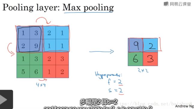
• max pooling, most used. works great. No one knows exactly why, maybe choose out the strongest feature
• average pooling: much less used

• pooling applies to each of your channels independently
• there is no parameters to learn in pooling layer, it’s just a fixed layer. Only hyperparameters to set.

Lecture 010: Convolutional neural network example

• A CNN example, inspired by LeNet-5
• notation: only layers with parameters is regarded as layers, so pooling layer is added to conv layer.
• a max-pooling of size $f=2,s=2$ will shrink the size of origin size $(W,H)$to $(W/2,H/2)$
• And I know this seems like there are a lot of hyperparameters, we’ll give you some more specific suggestions later for how to choose these types of hyperparameters. Maybe one common guideline is to actually not try to invent your own settings of hyperparameters, But to look in the literature to see what hyperparameters that work well for others. And just choose an architecture that has worked well for someone else, and there’s a chance that will work for your application as well.
• As you go deeper in NN, usually the $n_H,n_W$ will decrease, will the number of channels $n_c$ will increase.

• most CNNs have similar properties/ patterns to above ones
• A CNN, the CONV layer, the POOLING layer, and the fully connected layer. A lot of CV research has gone into figuring out how to put together these basic building blocks to build effective neural networks, and putting these things together actually requires quite a bit of insight. I think that one of the best ways for you to gain intuition about how to put these things together is to see a number of concrete examples of how others have done it.

011. Why convolutions?

• see the origin, filter, and output. if we build a linear fully connections, we are going to have $4704\times 3072+4704\approx 14M$ parameters. But if we use a conv filter, the number of parameters shrinked to $5\times 5\times 6+6=156$. A giant progress.
  

• Why conv so efficient? There are two main reasons

  • Parameter sharing: A feature detector (a low-level edge detector, or a high-level eye detector) that’s useful in one part of the image is probably useful in other part of the image.
  • Sparsity of connections: In each layer, each output value depends only on a small number of inputs. 卷积的响应值只和 filter 覆盖的那一块儿区域有关, 而与其他区域无关. Sparisity.

• Putting it together
  

Week 02: Case Studies

Lecture 001: Why look at case studies?

I think that a good way to get an intuition of how to build components is to read or to see other examples of effective components. And it turns out that a NN architecture that works well on one CV task often works well on other tasks as well.

• classic networks: build the foundation
  • LeNet-5
  • AlexNet
  • VGG
• ResNet(152 layers deep, good experience of trainning such a deep model)
• Inception

Lecture 002: Classic networks

• LeNet - 5, designed by LeCun et al. was aimed for digital numbers recognition on 32x32x1 gray images. Very primal architecture for CNN evolution
  

• AlexNet

DL was starting to gain attraction in speech recognition and a few other areas, but it was really this paper that convinced a lot of the CV community to take a serious look at DL and to convince them that DL did work well in CV and then it grew on to have a huge impact.

• VGG-16
  • simple repetive architecture, CONV = 3x3 filter, s=1, same. MAX-POOL=2x2, s=2
  • goes very deep
  • ~138M parameters
    

Lecture 003: Residual Networks(ResNets)

ResNet is designed to train very deep network by adding short-cuts to plain networks.

• 极大的优势就是，
  • in theory, the deeper, the smaller error
  • but in practice, is a U curve
  • but ResNet did achieve that theory perfomance

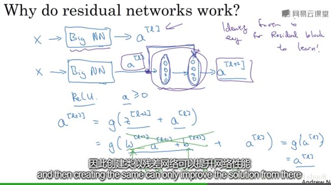
Lecture 004: Why ResNets work so well?

• Very good at identity formation learning. Skip the layer
  

Lecture 005: Network in Network and 1x1 convolutions

• could be used to shrink/keep/increase the #channels of your volumn

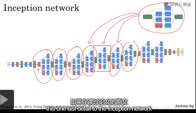
Lecture 006: Inception network motivation

If you’re building a layer of a NN, and you don’t have to decide do you want a 1x1 or 3x3 or 5x5 of pooling layer, the inception module, let’s you say, let’s do them all, and let’s concatenate the results.
Huge amout of compution could be shrinked to 1/10 using a well-designed bottomneck with 1x1 convolutions.

Lecture 007: Inception Network

• Inception module
  

• GoogLeNet
  

Lecture 008: Using open-source implementations

Lecture 009: Transfer Learning

• Transfer other’s model to train mine using a small set of data

Lecture 010:

V. 序列模型

---

Ref

• 吴恩达deeplearning.ai学完总结 : 很用心了. 给我的学习计划和体例安排带来很大的启发.