攻城狮成长日志(八):CRF+LSTM联手解决NER任务.

条件随机场(CRF)简介

讲到CRF,你就不得不谈一谈HMM,他们同属于概率图模型且建模的思想大致相同,而且已经有人证明了CRF其实就是无向图版的HMM.

但是,同时他们也存在着不同点.HMM属于生成式模型,而CRF则属于判别式模型,当然他们最大的不同还是对应的训练方式,CRF能根据具体的序列任务来调节模型,而HMM仅仅计算的是统计后的数据.因此也说CRF是升级版的HMM.

首先我们来看一看他们的公式表示,由上一节我们知道对于HMM公式有:
$$P(x,y)=P(y_1|start)\prod _{t=1}^{L-1}P(y_{t+1}|y_t)P(end|y_t)\prod _{t=1}^{L}P(x_t|y_t)$$

而对于CRF他的公式表达则为:
$$P(x,y)\propto exp(W\ast \varphi (x,y))$$
而$\varphi (x,y)$的意思就是指对应的词x被标示词性y的次数,我们可以记做$N(x,y)$,那么其实对应于一句话如The dog ate the homework且其对应的标注为D N V D N我们可以得到他对应的$\varphi (x,y)$由两部分,第一部分是标签和字词间的关系,记录如下:

Part1	Value
D, the	2
D, dog	0
…	…
N, the	0
N, dog	1
…	…
V, the	0
V, dog	0
…	…

而第二部分则是标签间的统计关系记录如下:

Part2	Value
D, D	0
D, V	0
…	…
N, N	0
N, V	1
…	…
V, V	0
V, D	1
…	…

这两部分统一起来就叫做序列标注任务的特征向量.而且十分有趣的是,你甚至可以自定义这个特征向量,来实现你期望达到的效果.

条件随机场的训练

对于给定的训练数据$(X,Y)$我们期待找到一个最大的$w^{\prime }$来满足如下的公式:
$$\begin{gathered} w^{\prime }=argma{x}_{w}O(w) \\ O(w)=\sum _{n=1}^{N}logP(y^{\prime n}|x^n)=logP(x^n,y^{\prime n})-log\sum _{y^{\prime }}P(x^n,y^{\prime }) \end{gathered}$$
可以看到我们同时期望最大化在序列中出现过的序列组合也就是$logP(x^n,y^{\prime n})$而另外的我们也要最小化在文本中没有出现过的转移组合也就是$log{\sum }_{y^{\prime }}P(x^n,y^{\prime })$

而对应的优化方法,容易想到可以采用类似梯度下降的方法,只不过由于我们是最大化函数,所以称作梯度上升.对应的梯度计算较为复杂,这里只给出最后的梯度计算出来是多少,公式如下:
$$\Delta w=N(x^n,y^{\prime n})-\sum _{y^{\prime }}P(y^{\prime }|x^n)N(x^n,y^{\prime })$$
在计算后一项时,其实复杂度十分的大,这里的计算方法涉及到维特比算法,就不深入讨论了.

LSTM解决NER问题

其实对应于NER任务,我们也可以用LSTM来进行解决.如下图我们可以得到一个序列的结果:
但是也很有可能出现上述的三个D连续出现的情况,这明显是不符合实际的.

CRF+LSTM联手解决

那么考虑到LSTM强大的可塑性,同时CRF的强大的可解释性,那么很容易就会想到吧这两个模型结合一下,自然就可以得到更好的结果了呀.

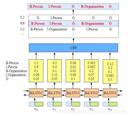
为了更好的性能,LSTM这里采用的是双向LSTM.那么这时候就能让我们的模型更可靠了.

代码实战

最后的代码不仅包含了前一节的HMM的代码,还包括了对应的单个CRF,LSTM以及对应的BiLSTM和CRF的组合模型.

import warnings
from itertools import zip_longest

from sklearn_crfsuite import CRF
import pandas as pd
import numpy as np
import torch
from torch import nn
from torch.nn.utils.rnn import pack_padded_sequence, pad_packed_sequence
import torch.nn.functional as F

warnings.filterwarnings('ignore')


def Load_Data(filepath, build_dict=True):
    # 读取对应的数据
    wordlists = []
    taglists = []
    with open(filepath, 'r', encoding='utf-8') as f:
        wordlist = []
        taglist = []
        for line in f:
            if line != '\n':
                # 如果不是回车符则属于同一句话
                word, tag = line.strip('\n').split()
                wordlist.append(word)
                taglist.append(tag)
            else:
                # 否则当作别的一段话添加到文档中
                wordlists.append(wordlist)
                taglists.append(taglist)
                wordlist = []
                taglist = []
    if build_dict:
        word2id = Build_Dict(wordlists)
        tag2id = Build_Dict(taglists)
        # 将字转换成对应的字典
        return wordlists, taglists, word2id, tag2id
    else:
        return wordlists, taglists


def Build_Dict(lists):
    dic = {}
    for list in lists:
        list_set = set(list)
        for letter in list_set:
            if letter not in dic.keys():
                dic[letter] = len(dic)
    return dic


class HMM(object):
    def __init__(self, N, M):
        """
        隐马尔可夫模型
        :param N: 状态数即对应的隐藏标注种类
        :param M: 观测数即对应的字数
        """
        self.N = N
        self.M = M
        self.A = torch.zeros(N, M)  # 状态转移矩阵
        self.B = torch.zeros(N, M)  # 发射概率矩阵
        self.Pi = torch.zeros(N)  # 初始状态矩阵

    def train(self, word_lists, tag_lists, word2id, tag2id):
        """
        对应隐马的训练过程，其实是统计的过程
        :param word_list:   列表，其中每个元素由字组成的列表，如 ['担','任','科','员']
        :param tag_list:  列表，其中每个元素是由对应的标注组成的列表，如 ['O','O','B-TITLE', 'E-TITLE']
        :param word2id: 将字映射为ID
        :param tag2id:  字典，将标注映射为ID
        :return:
        """

        assert len(word_lists) == len(tag_lists)  # 用于判断对应的每一个观测状态是否都有对应的隐藏状态

        # 统计概率转移矩阵
        for tag_list in tag_lists:
            # 统计状态转换矩阵
            seq_len = len(tag_list)
            for i in range(seq_len - 1):
                current_tagid = tag2id[tag_list[i]]
                next_tagid = tag2id[tag_list[i + 1]]
                self.A[current_tagid][next_tagid] += 1

            # 统计初始状态矩阵
            init_tag = tag_list[0]
            init_tagid = tag2id[init_tag]
            self.Pi[init_tagid] += 1

        # 估计发射概率矩阵
        for i in range(len(word_lists)):
            word_list = word_lists[i]
            tag_list = tag_lists[i]
            assert len(word_list) == len(tag_list)
            for j in range(len(word_list)):
                tag_list2id = tag2id[tag_list[j]]
                word_list2id = word2id[word_list[j]]
                self.B[tag_list2id][word_list2id] += 1

        # 避免为0，添上一个极小数
        self.A[self.A == 0] = 1e-10
        self.A = self.A / self.A.sum(dim=1, keepdim=True)

        self.Pi[self.Pi == 0] = 1e-10
        self.Pi = self.Pi / self.Pi.sum()

        self.B[self.B == 0] = 1e-10
        self.B = self.B / self.B.sum(dim=1, keepdim=True)

    def decoding(self, word_list, word2id, tag2id):
        """
        维特比算法查找最佳的序列.
        :param word_lists:
        :param word2id:
        :param tag2id:
        :return:
        """
        # 将相乘转换成相加避免下溢
        logA = torch.log(self.A)
        logB = torch.log(self.B)
        logPi = torch.log(self.Pi)
        seq_len = len(word_list)
        # 初始化维特比矩阵，维度（状态数*序列长度)
        Viterbi = torch.zeros(self.N, seq_len)

        # 解码回溯时使用
        # backPoints[i, j]存储的是 标注序列的第j个标注为i时，第j-1个标注的id
        backPoints = torch.zeros(self.N, seq_len)

        # 计算初始的转换选择的概率为多少
        BT = logB.t()  # 将B转置
        start_wordid = word2id.get(word_list[0], None)
        if not start_wordid:
            # 如果该词不在字典中则默认发射概率为均值
            bt = torch.log(torch.ones(self.N) / self.N)
        else:
            # 否则计算对应的词id，同时获取对应的B中可能转移到初始词的所有隐藏状态bt
            bt = BT[start_wordid]
        # 所有初始隐藏状态出现概率Pi 再加上 从初始隐藏状态发射到对应词和字的概率.
        Viterbi[:, 0] = logPi + bt
        backPoints[:, 0] = -1

        # 递推公式: 维特比第step的tag_id的状态等于step-1步的所有隐藏状态,
        # 乘以step-1步隐藏状态转移到step步的条件概率，
        # 再乘以对应step步发射到对应词的条件概率
        # Viterbi[tag_id, step] = max(Viterbi[: , step-1] * self.A.T()[tag_id] * Bt[word]
        for step in range(1, seq_len):
            word_id = word2id.get(word_list[step], None)
            if not word_id:
                bt = torch.log(torch.ones(self.N) / self.N)
            else:
                bt = BT[word_id]
            for tag_id in range(len(tag2id)):
                max_prob, max_id = torch.max(Viterbi[:, step - 1] + logA[:, tag_id], dim=0)
                Viterbi[tag_id, step] = max_prob + bt[tag_id]
                backPoints[tag_id, step] = max_id

        # 找到最后的标签并回溯
        best_path_prob, best_path_pointer = torch.max(
            Viterbi[:, seq_len - 1], dim=0
        )

        best_path_pointer = best_path_pointer.item()
        best_path = [best_path_pointer]
        for back_step in range(seq_len - 1, 0, -1):
            best_path_pointer = backPoints[best_path_pointer, back_step]
            best_path_pointer = int(best_path_pointer.item())
            best_path.append(best_path_pointer)

        # 将标签转换成字词
        assert len(best_path) == seq_len
        id2tag = dict((id, tag) for tag, id in tag2id.items())
        tag_path = [id2tag[id] for id in reversed(best_path)]
        return tag_path


class CRFmodel(object):
    def __init__(self):
        self.model = CRF(algorithm='lbfgs',
                         c1=0.1,
                         c2=0.2,
                         max_iterations=100,
                         all_possible_transitions=False
                         # 该项用于选择是机器自动生成标签集合还是用我们自定义的
                         )

    def train(self, sentences, tag_lists):
        """
        训练模型，
        :param sentences:
        :param tag_lists:
        :return:
        """
        features = [self.seq2features(s) for s in sentences]
        self.model.fit(features, tag_lists)

    def test(self, sentences):
        """
        预测测试集合数据
        :param sentences:
        :param tag_lists:
        :return:
        """
        features = [self.seq2features(s) for s in sentences]
        return self.model.predict(features)

    # 定义为类方法，以便不必要生成实例去调用该方法
    def word2features(self, seq, i):
        """抽取单词的特征函数"""
        word = seq[i]
        prev_word = "" if i == 0 else seq[i - 1]
        next_word = "" if i == (len(seq) - 1) else seq[i + 1]
        # 因为每个词相邻的词会影响这个词的标记
        # 所以我们使用：
        # 前一个词，当前词，后一个词，
        # 前一个词+当前词， 当前词+后一个词  五项作为特征
        feature = {
            'w': word,
            'w-1': prev_word,
            'w+1': next_word,
            'w-1:w': prev_word + word,
            'w:w+1': word + next_word,
            'bias': 1
        }
        return feature

    # 定义为类方法，以便不必要生成实例去调用该方法
    def seq2features(self, seq):
        """提取对应的序列特征"""
        return [self.word2features(seq, i) for i in range(len(seq))]


class BiLSTM(nn.Module):
    def __init__(self, args):
        super(BiLSTM, self).__init__()
        self.args = args

        # 将特定长的one—hot词向量转换成对应的输入维度
        self.embedding = nn.Embedding(self.args["vocabsize"], self.args["input_dim"])

        # 定义LSTM网络的输入，输出，层数，是否batch_first，dropout比例，是否双向
        self.BiLSTM = nn.LSTM(input_size=self.args["input_dim"],
                              hidden_size=self.args["hidden_dim"],
                              num_layers=self.args["num_layers"],
                              dropout=self.args["dropout"],
                              bidirectional=self.args["bidirectional"],
                              batch_first=True
                              )

        # 添加线性层,双向记得将维度修改为2*hidden_dim.
        self.Linear = nn.Linear(in_features=2 * self.args["hidden_dim"],
                                out_features=self.args["output_dim"])

    def forward(self, x, lengths):
        # 此处的lengths对应的是batchx里面每一个的长度,故不能提前设定
        embedding_x = self.embedding(x)
        packed_x = pack_padded_sequence(embedding_x, lengths, batch_first=True)
        packed_x, _ = self.BiLSTM(packed_x)
        x, _ = pad_packed_sequence(packed_x, batch_first=True)
        x = self.Linear(x)
        # 到这里要将对应的几率转换成序列，默认是采用最大的一个序列作为输出.
        return x

    def test(self, x, lengths):
        # test区别开训练和非训练的情况，可以使得不必要转换成对应的标签
        x = self.forward(x, lengths)
        _, tagid = torch.max(x, dim=2)
        return tagid


def extend_maps(word2id, tag2id, for_crf=True):
    # 用于对word2id和tag2id进行扩充
    word2id[''] = len(word2id)
    word2id[''] = len(word2id)
    tag2id[''] = len(tag2id)
    tag2id[''] = len(tag2id)
    if for_crf:
        word2id[''] = len(word2id)
        word2id[''] = len(word2id)
        tag2id[''] = len(tag2id)
        tag2id[''] = len(tag2id)
    return word2id, tag2id


def cal_lstm_loss(logits, targets, tag2id):
    # logits是对应预测的结果，targets是对应的预测标签集合
    PAD = tag2id.get('')
    assert PAD is not None

    # 筛选掉所有的因为补位而插入的PAD，使其不参与最后的运算.
    mask = (targets != PAD)
    targets = targets[mask]
    out_size = logits.size(2)

    # unsqueeze添加第三个维度
    mask = mask.unsqueeze(2)
    # 同时扩展mask尺寸成维度[B,L,out_size]
    mask = mask.expand(-1, -1, out_size)
    # mask_select选择对应的被遮盖的元素出来.
    logits = logits.masked_select(mask)
    # 因为view需要tensor的内存是整块的 所以调用contiguous()连续存储
    logits = logits.contiguous()
    # 然后用View转变维度到二维
    logits = logits.view(-1, out_size)

    assert logits.size(0) == targets.size(0)
    # 最后的targets维度[B*L]，而logits则是维度为[B*L, outsize]，调用后端计算值即可.
    loss = F.cross_entropy(logits, targets)
    return loss


class BiLSTM_CRF(nn.Module):
    def __init__(self, args):
        super(BiLSTM_CRF, self).__init__()

        # 设置一个前面的LSTM模型先。
        self.BiLSTM = BiLSTM(args)

        # CRF为对应的转移矩阵,维度[L,L],数字为1/output_dim
        self.Transition = nn.Parameter(torch.ones(args["output_dim"], args["output_dim"]) * 1 / args["output_dim"])

    def forward(self, x, lengths):
        # x的维度是[B, L, output_dim],output_dim其实就是标签个数
        x = self.BiLSTM(x, lengths)
        batch_size, max_len, out_size = x.size()
        # [B,L,output_dim,output_dim] + [1, output_dim, output_dim],
        # 容易明白[1,output_dim,output_dim]其实是标签间相互转换的概率
        crf_Score = x.unsqueeze(2).expand(-1, -1, out_size, -1) + self.Transition.unsqueeze(0)
        return crf_Score

    def Decode(self, data, tag2id, lengths):
        # 对应的是转换过后的tensor，标签转
        start_id = tag2id['']
        end_id = tag2id['']
        pad = tag2id['']
        tagset_size = len(tag2id)  # 总共的标签数

        crf_score = self.forward(data, lengths)

        # 获取对应维度的信息:Batchsize, Length, Target
        B, L, T, _ = crf_score.size()

        # 记录最大转移概率的矩阵, viterbi[i, j, k]表示第i个句子，第j个字对应第k个标记的最大分数
        viterbi = torch.zeros(B, L, T)

        # 对应回溯计算标签时候的矩阵
        backPointer = (torch.zeros(B, L, T).long() * end_id)

        length = torch.LongTensor(lengths)
        # 前馈过程
        for step in range(L):
            batch_size_t = (length > step).sum().item()
            if step == 0:
                # 起始转换状态。
                viterbi[:batch_size_t, step, :] = crf_score[:batch_size_t, step, start_id, :]
                # backpointer记录对应的标签状态
                backPointer[:batch_size_t, step, :] = start_id
            else:
                max_scores, prev_tag = torch.max(viterbi[:batch_size_t, step - 1, :].unsqueeze(2) +
                                                 crf_score[:batch_size_t, step, :, :], dim=1)
                viterbi[:batch_size_t, step, :] = max_scores
                backPointer[:batch_size_t, step, :] = prev_tag

        # 回馈过程采用backPointer实现
        backPointer = backPointer.view(B, -1)  # 改变维度
        tagids = []  # 记录最后的标签序列
        tags_t = None
        for step in range(L - 1, 0, -1):
            batch_size_t = (length > step).sum().item()
            if step == L - 1:
                # 如果是最后一步
                index = torch.ones(batch_size_t).long() * (step * tagset_size)
                index += end_id
            else:
                prev_batch_size_t = len(tags_t)
                new_in_batch = torch.LongTensor([end_id] * (batch_size_t - prev_batch_size_t))
                offset = torch.cat(
                    [tags_t, new_in_batch],
                    dim=0
                )
                index = torch.ones(batch_size_t).long() * (step * tagset_size)
                index += offset.long()

            tags_t = backPointer[:batch_size_t].gather(
                dim=1,
                index=index.unsqueeze(1).long())
            tags_t = tags_t.squeeze(1)
            tagids.append(tags_t.tolist())
        tagids = list(zip_longest(*reversed(tagids)), fillvalue=pad)
        tagids = torch.Tensor(tagids).long()
        return tagids


class Metrics:
    def __init__(self, x, y, label):
        self.x = x
        self.y = y
        self.label = label
        self.correctEntity = 0  # 正确预测出来的实体
        self.labelEntity = 0  # 样本实体数
        self.predictEntity = 0  # 识别实体数
        self.Cal_Entity()

    def Cal_Entity(self):
        # 计算对应的correctEntity,labelEntity,predictEntity三类实体的数目
        assert len(self.y) == len(self.label)
        for i in range(len(self.y)):
            assert len(self.y[i]) == len(self.label[i])
            # 逐个比对对应的标签状态
            tem_predict = self.Split(self.x[i], self.y[i])
            tem_label = self.Split(self.x[i], self.label[i])
            for e in tem_predict:
                if e in tem_label:
                    self.correctEntity += 1
            self.labelEntity += len(tem_label)
            self.predictEntity += len(tem_predict)

    def F1_Measure(self):
        presicion = self.correctEntity / self.predictEntity
        recall = self.correctEntity / self.labelEntity
        return (2 * presicion * recall) / (recall + presicion)

    def Accuracy(self):
        return self.correctEntity / self.predictEntity

    def Split(self, x, y):
        # 精确匹配分割对应的实体集
        i = 0
        strings = []
        while i < len(y):
            string = ""
            if y[i][0] == 'B':
                # 匹配到开头则分割词
                while i < len(y) and y[i][0] != 'E':
                    string += x[i]
                    i += 1
                string += x[i]
            else:
                i += 1
            if string:
                strings.append(string)
        return strings


def tensorized(batch, maps):
    # batch是对应的文字,maps是对应的映射
    PAD = maps.get('')
    UNK = maps.get('')
    # 排好序列的所以取第一个
    max_len = len(batch[0])
    batch_size = len(batch)
    batch_tensor = torch.ones(batch_size, max_len).long() * PAD
    for i, l in enumerate(batch):
        for j, e in enumerate(l):
            batch_tensor[i][j] = maps.get(e, UNK)
    # batch各个元素的长度
    lengths = [len(l) for l in batch]
    return batch_tensor, lengths


def sort_by_lengths(word_lists, tag_lists):
    # 按照长度从大到小排序好
    pairs = list(zip(word_lists, tag_lists))
    indices = sorted(range(len(pairs)),
                     key=lambda k: len(pairs[k][0]),
                     reverse=True)
    pairs = [pairs[i] for i in indices]

    word_lists, tag_lists = list(zip(*pairs))

    return word_lists, tag_lists  # , indices


def prepocess_data_for_lstmcrf(word_lists, tag_lists, test=False):
    # 将LSTM-CRF的数据尾部添上对应的
    assert len(word_lists) == len(tag_lists)
    for i in range(len(word_lists)):
        word_lists[i].append("")
        if not test:  # 如果是测试数据，就不需要加end token了
            tag_lists[i].append("")

    return word_lists, tag_lists


def cal_lstm_crf_loss(crf_scores, targets, tag2id):
    """计算双向LSTM-CRF模型的损失
    crf_scores:[B,L,output_dim,output_dim]
    该损失函数的计算可以参考:https://arxiv.org/pdf/1603.01360.pdf
    """
    pad_id = tag2id.get('')
    start_id = tag2id.get('')
    end_id = tag2id.get('')

    # targets:[B, L] crf_scores:[B, L, T, T]
    batch_size, max_len = targets.size()
    target_size = len(tag2id)

    # mask = 1 - ((targets == pad_id) + (targets == end_id))  维度为:[B, L]
    # 遮盖掉为pad也就是不参与计算的或者是为终止符号的
    mask = (targets != pad_id)
    lengths = mask.sum(dim=1)
    targets = indexed(targets, target_size, start_id)

    # 计算Golden scores方法１
    # golden scores...高分的意思，也就意思是找出整个转移矩阵中最高分的排列...
    targets = targets.masked_select(mask)  # [real_L]

    #从预测结果中选择所有未被遮盖的，然后转换成对应目标的形式.
    flatten_scores = crf_scores.masked_select(
        mask.view(batch_size, max_len, 1, 1).expand_as(crf_scores)
    ).view(-1, target_size * target_size).contiguous()

    #记分方式,这个是对应的正确序列的分数
    golden_scores = flatten_scores.gather(
        dim=1, index=targets.unsqueeze(1)).sum()

    # 计算golden_scores方法２：利用pack_padded_sequence函数
    # targets[targets == end_id] = pad_id
    # scores_at_targets = torch.gather(
    #     crf_scores.view(batch_size, max_len, -1), 2, targets.unsqueeze(2)).squeeze(2)
    # scores_at_targets, _ = pack_padded_sequence(
    #     scores_at_targets, lengths-1, batch_first=True
    # )
    # golden_scores = scores_at_targets.sum()

    # 计算all path scores,整个过程类似于维特比算法。t时间都是基于t-1时间计算的.
    # scores_upto_t[i, j]表示第i个句子的第t个词被标注为j标记的所有t时刻事前的所有子路径的分数之和
    scores_upto_t = torch.zeros(batch_size, target_size)
    for t in range(max_len):
        # 当前时刻 有效的batch_size（因为有些序列比较短)
        batch_size_t = (lengths > t).sum().item()
        if t == 0:
            # 第一步是直接复制所有初始步分数
            scores_upto_t[:batch_size_t] = crf_scores[:batch_size_t, t, start_id, :]
        else:
            # 将当前步的分数加到现在总计的分数里,为取消乘法，先取对数相加在取指数。
            # 上一个时间步的cur_标记是此时间步的prev_标记
            # 所以，广播PREV。timestep的cur_标记沿cur得分。时间步的cur_标记维度
            scores_upto_t[:batch_size_t] = torch.logsumexp(
                crf_scores[:batch_size_t, t, :, :] +
                scores_upto_t[:batch_size_t].unsqueeze(2),
                dim=1
            )
    #最后对所有最大路径的分数进行求和
    all_path_scores = scores_upto_t[:, end_id].sum()

    # 训练大约两个epoch loss变成负数，从数学的角度上来说，loss = -logP
    loss = (all_path_scores - golden_scores) / batch_size
    return loss


def indexed(targets, tagset_size, start_id):
    """将targets中的数转化为在[T*T]大小序列中的索引,T是标注的种类"""
    batch_size, max_len = targets.size()
    for col in range(max_len - 1, 0, -1):
        targets[:, col] += (targets[:, col - 1] * tagset_size)
    targets[:, 0] += (start_id * tagset_size)
    return targets


if __name__ == '__main__':
    filedir = "/Users/XYJ/Downloads/LatticeLSTM-master/data/"
    filenames = ["demo.train.char", "demo.test.char", "demo.dev.char"]
    wordlists, taglists, word2id, tag2id = Load_Data(filedir + filenames[0])  # 对应的训练集标签样例
    # 在获取测试集的时候是不需要获取对应的标签的因为可能存在标签集比原先小的情况
    test_wordlists, test_taglists = Load_Data(filedir + filenames[2], build_dict=False)  # 对应的测试样例的标签

    # -----------------HMM训练
    # MyHMM = HMM(len(tag2id), len(word2id))
    # MyHMM.train(wordlists, taglists, word2id, tag2id)
    # alltagpath = []
    # for i in range(len(test_wordlists)):
    #     tagpath = MyHMM.decoding(test_wordlists[i], word2id, tag2id)
    #     alltagpath.append(tagpath)
    # HMM_metrics = Metrics(test_wordlists, alltagpath, test_taglists)
    # print("Accuracy:{}".format(HMM_metrics.Accuracy()))

    # -----------------CRF训练
    # MyCRF = CRFmodel()
    # MyCRF.train(wordlists, taglists)
    # alltagpath = MyCRF.test(test_wordlists)
    # CRF_metrics = Metrics(test_wordlists, alltagpath, test_taglists)
    # print(CRF_metrics.Accuracy())

    # -----------------LSTM训练
    # 添加特殊标识符和,因此必须在创建模型前拓展哦！
    # word2id, tag2id = extend_maps(word2id, tag2id, for_crf=False)
    # args = {
    #     "vocabsize": len(word2id),  # 对应词个数
    #     "input_dim": 128,  # 词向量嵌入维度
    #     "hidden_dim": 64,  # 隐藏层的维度
    #     "num_layers": 1,  # 层数
    #     "dropout": 0.1,
    #     "bidirectional": True,  # 是否构成双向
    #     "output_dim": len(tag2id),  # 对应标签的个数
    # }
    # BATCHSIZE = 32

    # # 定义损失函数,优化器
    # MyLSTM = BiLSTM(args)
    # optimizer = torch.optim.Adam(MyLSTM.parameters(), lr=0.02)
    #
    # 需要将文字wordlist按大小排序,方便后面转换
    # wordlists, taglists = sort_by_lengths(wordlists, taglists)
    #
    # for epoch in range(10):
    #     loss = 0
    #     for ind in range(0, len(wordlists), BATCHSIZE):
    #         # 每次输入BATCHSIZE个句子同时因为已经按照句子长度排序了。故只取第一个为最大的。
    #         batch_sent, batch_tags = wordlists[ind:ind + BATCHSIZE], taglists[ind:ind + BATCHSIZE]
    #
    #         # 再按照Batchsize逐个读入转换成对应的数字先
    #         tensorized_tensor, lengths = tensorized(batch_sent, word2id)
    #
    #         # 同样转换对应的tags,两个lengths都一样的.
    #         targets, _ = tensorized(batch_tags, tag2id)
    #
    #         # forward过程
    #         prediction = MyLSTM(tensorized_tensor, lengths)
    #
    #         # 损失函数计算，梯度求导.----------------------------
    #         newloss = cal_lstm_loss(prediction, targets, tag2id)
    #         loss += newloss  # 损失累加
    #         optimizer.zero_grad()  # 梯度置零
    #         newloss.backward()  # 反馈
    #         optimizer.step()
    #
    #     # 输出对应的epoch和损失
    #     print("epoch:{},loss:{}".format(epoch, loss))
    #
    # # 对应的预测结果
    # tensorized_test_tensor, lengths = tensorized(test_wordlists, word2id)
    #
    # prediction = MyLSTM.test(tensorized_test_tensor, lengths)

    # ------------Bi-LSTM+CRF模型
    # 字典添加对应的和
    word2id, tag2id = extend_maps(word2id, tag2id, for_crf=True)
    # 句子添加上和
    wordlists, taglists = prepocess_data_for_lstmcrf(wordlists, taglists)
    # 测试数据同样处理.
    test_wordlists, test_taglists = prepocess_data_for_lstmcrf(test_wordlists, test_taglists, test=True)
    args = {
        "vocabsize": len(word2id),  # 对应词个数
        "input_dim": 128,  # 词向量嵌入维度
        "hidden_dim": 64,  # 隐藏层的维度
        "num_layers": 1,  # 层数
        "dropout": 0.1,
        "bidirectional": True,  # 是否构成双向
        "output_dim": len(tag2id),  # 对应标签的个数
    }
    BATCHSIZE = 32
    model = BiLSTM_CRF(args)
    optimizer = torch.optim.Adam(model.parameters(), lr=0.02)
    # 按长度排序
    wordlists, taglists = sort_by_lengths(wordlists, taglists)
    for epoch in range(10):
        loss = 0
        for ind in range(0, len(wordlists), BATCHSIZE):
            # 每次输入BATCHSIZE个句子同时因为已经按照句子长度排序了。故只取第一个为最大的。
            batch_sent, batch_tags = wordlists[ind:ind + BATCHSIZE], taglists[ind:ind + BATCHSIZE]

            # 再按照Batchsize逐个读入转换成对应的数字先
            tensorized_tensor, lengths = tensorized(batch_sent, word2id)

            # 同样转换对应的tags,两个lengths都一样的.
            targets, _ = tensorized(batch_tags, tag2id)

            # forward过程
            prediction = model(tensorized_tensor, lengths)

            # 损失函数计算，梯度求导.----------------------------
            newloss = cal_lstm_crf_loss(prediction, targets, tag2id)
            loss += newloss  # 损失累加
            optimizer.zero_grad()  # 梯度置零
            newloss.backward()  # 反馈
            optimizer.step()

        # 输出对应的epoch和损失
        print("epoch:{},loss:{}".format(epoch, loss))

总结

大致过了一边NER任务的基本内容,许多内容涉及到传统的概率图模型,同时代码也是比较难懂,但好歹还是坚持学完了,当然,大部分的代码都是从大佬的模型里面改写来的.只是站在巨人的肩膀上看了眼外面的世界.

参考文献

NLP实战-中文命名实体识别