降维算法之LDA及其实战

1.LDA介绍
      LDA（全称：Linear Discriminant Analysis，中文名称：线性判别分析）是一种有监督学习的降维技术，也就是说它的数据集的每个样本是有类标签的。Ronald A. Fisher在1936年提出了线性判别方法。
      用途：数据预处理中的降维，分类任务。
      目标：LDA关心的是能够最大化类间区分度的坐标成分。将特征空间（数据集中的多维样本）投影到一个维度更小的k维子空间中，同时保持区分类别的信息。
      原理：我们要将数据在低维度上进行投影，投影后希望每一种类别数据的投影点尽可能的接近，而不同类别的数据的类别中心之间的距离尽可能的大。（可以总结为LDA更关心分类，分类效果好了，类内的方差也就很小，类间的方差也就很大了。）

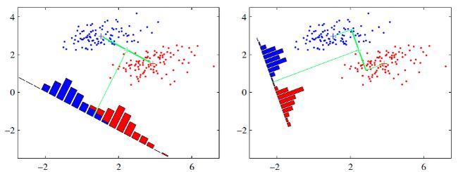
      从直观上可以看出，右图要比左图的投影效果好，因为右图的红色数据和蓝色数据各个较为集中，且类别之间的距离明显。左图则在边界处数据混杂。
2.数学原理（仅以二分类为例）

      目标：找到该投影 $$y=w^{T}x$$
      LDA分类的目标：使得不同类别之间的距离越远越好，同一类别之中的距离越近越好。
      每类样例的均值：$${\mu }_i=\frac{1}{N_i}\sum _{x\in w_i}x$$
      投影后的均值： $${\mu }_i=\frac{1}{N_i}\sum _{y\in w_i}y=\frac{1}{N_i}\sum _{x\in w_i}{w}^{T}x=w^T{\mu }_i$$
      投影后的两类样本中心点尽量分离： $$J\left(w\right)=\left|{\mu }_1-{\mu }_2\right|=\left|w^T\left({\mu }_1-{\mu }_2\right)\right|$$

      当然，只最大化$J\left(w\right)$是不能满足的，X1的方向可以最大化$J\left(w\right)$，但是区分度不好，即类之间的距离不够大，而且类之间还有重叠。所以，光衡量类间是不够的，还需要衡量类内的，那么散列值指标就出来了，它表示样本点的密集程度，值越大，越分散，反之，越集中。
      同类之间应该越密集些： $${s_i}^2={\sum _{y\in w_i}\left(y-{\mu }_i\right)}^2$$
      所以最后的目标函数变为： $$J\left(w\right)=\frac{\left|{\mu }_1-{\mu }_2\right|}{{s_1}^2+{s_2}^2}$$
      散列值公式展开：$${s_i}^2={\sum _{y\in w_i}\left(y-{\mu }_i\right)}^2={\sum _{x\in w_i}\left(w^{T}x-w^T{\mu }_i\right)}^2=\sum _{x\in w_i}{w}^T\left(x-{\mu }_i\right){\left(x-{\mu }_i\right)}^{T}w$$
      散列矩阵(scatter matrices)： $${s_i}^2=\sum _{x\in w_i}\left(x-{\mu }_i\right){\left(x-{\mu }_i\right)}^T$$
      类内散布矩阵：$$s_w=s_1+s_2$$
      则$${s_i}^2=w^T{s}_{i}w$$ $${s_1}^2+{s_2}^2=w^T{s}_{w}w$$
      分子展开：

       其中$s_B$称为类间散布矩阵。

      最终目标函数： $$J\left(w\right)=\frac{w^T{s}_{B}w}{w^T{s}_{w}w}$$
      分母归一化：如果分子、分母都是可以取任意值的，那就会产生无穷解，我们将分母的大小限制小于等于1。
      最终目标函数实际上越大越好，也就是，我们希望取得这个函数的极大值，极大值的求取，我们是不是想到了拉格朗日这个神器。下面就用此方法进行求解。
      拉格朗日乘子法：
$$c\left(w\right)=w^T{s}_{B}w-\lambda \left(w^T{s}_{w}w-1\right)$$
$$\Rightarrow \frac{dc}{dw}=2s_{B}w-2\lambda s_{w}w=0$$
$$\Rightarrow s_{B}w=\lambda s_{w}w$$

      两边都乘以$s_w$的逆：${s_w}^{-1}{s}_{B}w=\lambda w$（w就是矩阵${s_w}^{-1}{s}_B$的特征向量）
3.LDA实战（多分类为例，并将相关多分类所用到的公式附上）
3.1获取鸢尾花数据集

feature_dict = {i:label for i,label in zip(
                range(4),
                  ('sepal length in cm',
                  'sepal width in cm',
                  'petal length in cm',
                  'petal width in cm', ))}
import pandas as pd
df = pd.io.parsers.read_csv(
        filepath_or_buffer = 'https://archive.ics.uci.edu/ml/machine-learning-databases/iris/iris.data',
        header = None,
        sep = ','
    )
df.columns = [ l for i,l in sorted(feature_dict.items())] + ['class label']
# how='all’滤除全为NaN的行
df.dropna(how='all',inplace=True)
df.tail()

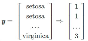
3.2将数据进行预处理，X表示特征，y表示标签

from sklearn.preprocessing import LabelEncoder

X = df[['sepal length in cm','sepal width in cm','petal length in cm','petal width in cm']].values
y = df['class label'].values

enc = LabelEncoder()
label_encoder = enc.fit(y)
y = label_encoder.transform(y) + 1

label_dict = {1: 'Setosa', 2: 'Versicolor', 3:'Virginica'}

      标签值进行了转化，转化后的结果为：

3.3分别求三种鸢尾花数据在不同特征维度上的均值向量 mi

import numpy as np
# 小数点后四位
np.set_printoptions(precision=4)

mean_vectors = []
for cl in range(1,4):
    mean_vectors.append(np.mean(X[y==cl],axis=0))
print('Mean Vector class %s: %s\n' %(cl, mean_vectors[cl-1]))

输出结果：

Mean Vector class 1: [5.006 3.418 1.464 0.244]
Mean Vector class 2: [5.936 2.77  4.26  1.326]
Mean Vector class 3: [6.588 2.974 5.552 2.026]

3.4计算两个 4×4 维矩阵：类内散布矩阵和类间散布矩阵
（1）类内散布矩阵
$$s_w=\sum _{i=1}^c{s}_i$$
$$s_i=\sum _{x\in D_i}^n\left(x-m_i\right){\left(x-m_i\right)}^T$$
$$m_i=\frac{1}{n_i}\sum _{x\in D_i}^n{x}_k$$
      $m_i$表示每一个类别的均值。

S_W = np.zeros((4,4))
for cl,mv in zip(range(1,4),mean_vectors):
    class_sc_mat = np.zeros((4,4))
    for row in X[y==cl]:
        row,mv = row.reshape(4,1),mv.reshape(4,1)
        class_sc_mat += (row-mv).dot((row-mv).T)
    S_W += class_sc_mat
print('within-class Scatter Matrix:\n', S_W)

输出结果：

within-class Scatter Matrix:
 [[38.9562 13.683  24.614   5.6556]
 [13.683  17.035   8.12    4.9132]
 [24.614   8.12   27.22    6.2536]
 [ 5.6556  4.9132  6.2536  6.1756]]

（2）类间散布矩阵
$$s_B=\sum _{i=1}^c{N}_i\left(m_i-m\right){\left(m_i-m\right)}^T$$
      m是全局均值，而mi和Ni是每类样本的均值和样本数。

overall_mean = np.mean(X,axis=0)

S_B = np.zeros((4,4))
for i,mv in enumerate(mean_vectors):
    n = X[y == i+1,:].shape[0]
    mv = mv.reshape(4,1)
    overall_mean = overall_mean.reshape(4,1)
    S_B += n * (mv - overall_mean).dot((mv - overall_mean).T)
    
print('between-class Scatter Matrix:\n', S_B)

输出结果：

between-class Scatter Matrix:
 [[ 63.2121 -19.534  165.1647  71.3631]
 [-19.534   10.9776 -56.0552 -22.4924]
 [165.1647 -56.0552 436.6437 186.9081]
 [ 71.3631 -22.4924 186.9081  80.6041]]

3.5求解矩阵的特征值（特征向量：表示映射方向；特征值的绝对值：特征向量的重要程度）

# linalg线性代数模块，eig求解特征值和特征向量，inv求解逆矩阵
eig_vals, eig_vecs = np.linalg.eig(np.linalg.inv(S_W).dot(S_B))

for i in range(len(eig_vals)):
    eigvec_sc = eig_vecs[:,i].reshape(4,1)
    print('\nEigenvector {}: \n{}'.format(i+1, eigvec_sc.real))
    print('Eigenvalue {:}: {:.2e}'.format(i+1, eig_vals[i].real))

输出结果：

Eigenvector 1: 
[[ 0.2049]
 [ 0.3871]
 [-0.5465]
 [-0.7138]]
Eigenvalue 1: 3.23e+01

Eigenvector 2: 
[[-0.009 ]
 [-0.589 ]
 [ 0.2543]
 [-0.767 ]]
Eigenvalue 2: 2.78e-01

Eigenvector 3: 
[[ 0.8767]
 [-0.2456]
 [-0.2107]
 [-0.356 ]]
Eigenvalue 3: -7.61e-16

Eigenvector 4: 
[[-0.7968]
 [ 0.4107]
 [ 0.4176]
 [-0.1483]]
Eigenvalue 4: 3.67e-15

（1）按特征值大小进行排序

eig_pairs = [(np.abs(eig_vals[i]), eig_vecs[:,i]) for i in range(len(eig_vals))]

# Sort the (eigenvalue, eigenvector) tuples from high to low
eig_pairs = sorted(eig_pairs, key=lambda k: k[0], reverse=True)

print('Eigenvalues in decreasing order:\n')
for i in eig_pairs:
print(i[0])

输出结果：

Eigenvalues in decreasing order:
32.27195779972982
0.2775668638400559
3.668801765648684e-15
7.606986544516927e-16

（2）衡量特征值的重要程度

print('Variance explained:\n')
eigv_sum = sum(eig_vals)

for i,j in enumerate(eig_pairs):
print('eigenvalue {0:}: {1:.2%}'.format(i+1, (j[0]/eigv_sum).real))

输出结果：

Variance explained:
eigenvalue 1: 99.15%
eigenvalue 2: 0.85%
eigenvalue 3: 0.00%
eigenvalue 4: 0.00%

（3）根据重要程度，选择前两维特征

W = np.hstack((eig_pairs[0][1].reshape(4,1), eig_pairs[1][1].reshape(4,1)))
print('Matrix W:\n', W.real)

输出结果：

Matrix W:
 [[ 0.2049 -0.009 ]
 [ 0.3871 -0.589 ]
 [-0.5465  0.2543]
 [-0.7138 -0.767 ]]

3.6降维

X_lda = X.dot(W)
assert X_lda.shape == (150,2), "The matrix is not 150x2 dimensional."

画图函数

import matplotlib.pyplot as plt
def plot_step_lda():
    
    ax = plt.subplot(111)
    for label,marker,color in zip(
        range(1,4),('^', 's', 'o'),('blue', 'red', 'green')):

        plt.scatter(x=X_lda[:,0].real[y == label],
                y=X_lda[:,1].real[y == label],
                marker=marker,
                color=color,
                alpha=0.5,
                label=label_dict[label]
                )
    plt.xlabel('LD1')
    plt.ylabel('LD2')
    
    leg = plt.legend(loc='upper right', fancybox=True)
    leg.get_frame().set_alpha(0.5)
    plt.title('LDA: Iris projection onto the first 2 linear discriminants')
    # hide axis ticks
    plt.tick_params(axis="both", which="both", bottom=False, top=False,  
            labelbottom=True, left=False, right=False, labelleft=True)

    # remove axis spines
    ax.spines["top"].set_visible(False)  
    ax.spines["right"].set_visible(False)
    ax.spines["bottom"].set_visible(False)
    ax.spines["left"].set_visible(False)    

    plt.grid()
    plt.tight_layout
    plt.show()

plot_step_lda()

3.7sklearn中的LDA降维

from sklearn.discriminant_analysis import LinearDiscriminantAnalysis as LDA

# LDA
sklearn_lda = LDA(n_components=2)
X_lda_sklearn = sklearn_lda.fit_transform(X,y)

      其结果和上面按照原理求解的一样。

参考文档：
https://www.cnblogs.com/pinard/p/6244265.html
https://blog.csdn.net/woaixuexihhh/article/details/85202077