无人驾驶二 卡尔曼滤波与PID控制
卡尔曼滤波形象的描述见:
https://blog.csdn.net/lybaihu/article/details/54943545
卡尔曼滤波与目标追踪示例见:
https://blog.csdn.net/AdamShan/article/details/78248421?locationNum=5&fps=1
清晰的推导见:
https://blog.csdn.net/heyijia0327/article/details/17487467
https://www.cnblogs.com/heguanyou/p/7502909.html
对差分方程:
![]()
![]()
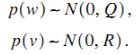
注意在离散状态空间方程中,测量方程稍微不同,先进行测量更新,再进行时间更新。


给空间状态参数赋值:
%Kalman filter
%x=Ax+B(u+w(k))
%y=Cx+D+v(k)
clear all;
close all;

TS=0.001;

%Continuous Plant to discrete-time Plant:
%sys=tf(133,[1,25,0]);
A=[0 1;0 -25];
B=[0;133];
C=[1 0];
D=[0];
[Ad,Bd,Cd,Dd]=c2dm(A,B,C,D,TS,'z');
卡尔曼滤波控制程序:
%Discrete Kalman filter
%x(k+1)=Ax(k)+B(u(k)+w(k));
%y(k)=Cx(k)+D+v(k)
function [u]=kalman(u1,u2,u3)
%u1:输入u
%u2:测量值yv
%u3:时间t
persistent A B C D Q R P x

yv=u2;
if u3==0
   TS=0.001;

   %Continuous Plant to discrete-time Plant:
    %sys=tf(133,[1,25,0]);
    A1=[0 1;0 -25];
    B1=[0;133];
    C1=[1 0];
    D1=[0];
    [A,B,C,D]=c2dm(A1,B1,C1,D1,TS,'z');

	%Covariances of w:
    Q=[0.1];

    %Covariances of v:
    R=[0.1];

    %初始估计值:
    x=zeros(2,1);

    %初始估计误差协方差:
    P=B*Q*B';
end

%后验,Measurement update:
%根据估计误差协方差和测量噪声协方差计算卡尔曼增益:
Kk=P*C'/(C*P*C'+R);

%计算最优估计值:
%x=A*x+Mn*(yv-C*A*x);%‘注意本处原文有误!!
x=x+Kk*(yv-C*x);

%计算最优估计值和真实值之间的误差协方差矩阵,为下次递推做准备:
P=(eye(2)-Kk*C)*P;

ye=C*x+D;           %Filtered value

u(1)=ye;    %Filtered signal
u(2)=yv;    %Signal with noise

errcov=C*P*C';      %Covariance of estimation error

%先验,Time update:
%根据系统状态方程计算下一状态预测值:
x=A*x+B*u1;
%预测误差协方差:
P=A*P*A'+B*Q*B';
绘图程序:
close all;
figure(1);
plot(t,y(:,1),'r',t,y(:,2),'k:','linewidth',2);
xlabel('time(s)');ylabel('y,ye');
legend('ideal signal','filtered signal');

figure(2);
plot(t,y(:,1),'r',t,y1(:,1),'k:','linewidth',2);
xlabel('time(s)');ylabel('y,yv');
legend('ideal signal','signal with noise');


注意:
If the plant model is direct feedthrough, this will result in an algebraic loop. While Simulink can solve the algebraic loop most of the time, it usually slows down the simulation.
If the blocks in the algebraic loop have a discrete sample time, inserting a Unit Delay is usually the best solution. Of course this will change the dynamic of the system, this is something you need to evaluate and see if this is acceptable for your application.
If the blocks in the loop have a continuous sample time, what many users try is inserting a Memory block. The Memory block is similar to the Unit Delay block in a sense that it delays its input by one time step, however it works with variable-step signals.
However when simulating the model, we quickly notice that it simulates very slowly
参考:
https://blogs.mathworks.com/simulink/2015/07/18/why-you-should-never-break-an-algebraic-loop-with-with-a-memory-block/
P=5; I=1; D=0.1; N=100;yd=sin(2*pi*0.05t)
不用卡尔曼滤波PID控制结果如下:
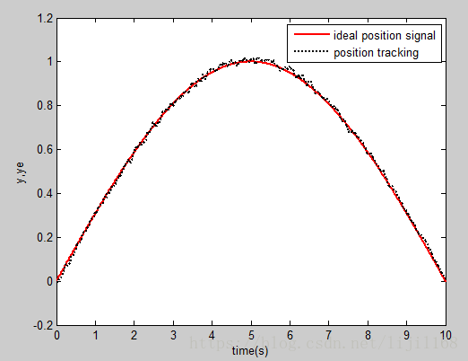
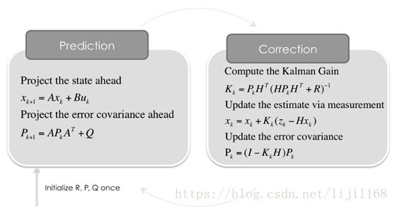
采用卡尔曼滤波后结果如下:
