零起点Tensorflow快速入门学习笔记（一）

目录

零起点Tensorflow快速入门学习笔记（一）

---

 

对第九章案例9-8进行了上级实验，根据书本提供的网址下载了代码和数据集。

主要改动如下：

一、关于建立自己的模块并引用

 源码中from libs.utils import *，这个因该是作者自己建立的模块，没有下载。于是自己尝试建立自己的模块。分析代码有3个函数：weight_variable(),bias_variable() and montage()。

实验了两种方式：

（一）

1.在源文件同目录下建立文件夹libs，而后在libs文件夹中建立两个文件__init__.py and utils.py;

2. __init__.py文件内容为空。只有文件夹包含此文件，此文件夹才被当作一个包。该文件内容可以为空，也可初始化一些变量等。

3.utils.py中包含3个函数，代码如下：

import tensorflow as tf

import numpy as np

'''解释说明'''

def weight_variable(shape):

    return tf.Variable(tf.truncated_normal(shape, dtype=tf.float32, stddev=1e-1), name='weights')

def bias_variable(shape):

    return tf.Variable(tf.constant(0.0, shape=shape, dtype=tf.float32))

def montage(s):

    temp = []

    for n in range(16):

        temp1 = []

        for j in range(5):

            for i in range(5):

                temp1.append(s[i][j][0][n])

            # print(temp1)

        t = np.reshape(temp1, (5, 5))

        print(t)

        temp.append(t)

    return temp

4.之后，就可以使用from libs.utils import *了。

（二）

1.在源文件同目录下建立文件夹libs/utils，而后在utils文件夹中建立4个文件__init__.py, weight_variable.py，bias_variable.py和montage.py

2.文件内容同上。将utils中的三个函数分别写到三个文件中。

3.注释掉from libs.utils import *，改为：

from libs.util.weight_variable import *

from libs.util.bias_variable import *

from libs.util.montage import *

运行即可。

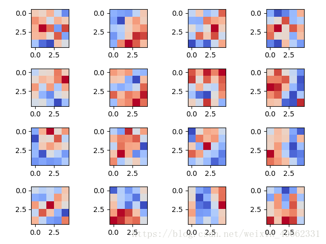
二、关于绘图的问题

代码如下：

print('\n#16,查看和权重卷积函数的示意图')

W = sess.run(W_conv1)

img=montage(W / np.max(W))

fig,ax=plt.subplots(4,4)

for i,axi in enumerate(ax.flat):

    axi.imshow(img[i],cmap='coolwarm')

plt.show()

三、关于pycharm中编辑代码时出现类似word中“改写”模式的问题，即光标变粗，插入字符会删除后续字符，可使用键盘“insert”键。

四、关于张量的问题

测试代码查看：

s=W / np.max(W) #s是4阶张量，其shape为[5,5,1,16]

print(len(s)) #5



print(len(s[0])) #5

print(s[0]) #3阶张量，其shape为[5,1,16]

print(len(s[0][0])) #1

print(s[0][0]) #2阶张量，其shape为[1,16]

print(len(s[0][0][0])) #16

print(s[0][0][0]) #1阶张量，其shape为[16]

print(s[0][0][1]) #提示错误，越界

print(s[0][1][0]) #1阶张量，其shape为[16]

print(s[0][1][0][0]) #0阶张量

附：

import tensorflow as tf
import tensorflow.examples.tutorials.mnist.input_data as input_data
from libs.utils import *
#from libs.util.weight_variable import *
#from libs.util.bias_variable import *
#from libs.util.montage import *
import numpy as np
import matplotlib.pyplot as plt

'''
def weight_variable(shape):
    return tf.Variable(tf.truncated_normal(shape, dtype=tf.float32, stddev=1e-1), name='weights')
def bias_variable(shape):
    return tf.Variable(tf.constant(0.0,shape=shape,dtype=tf.float32))
def montage(s):
    temp=[]
    for n in range(16):
        temp1 = []
        for j in range(5):
            for i in range(5):
                temp1.append(s[i][j][0][n])
            #print(temp1)
        t=np.reshape(temp1,(5,5))
        print(t)
        temp.append(t)
    return temp

'''


# -----------------------
# 1
print('\n#1,数据设置')
rlog = 'J:/tensorbord_test/mnist_study'
mnist = input_data.read_data_sets('j:/data/MNIST/', one_hot=True)
x = tf.placeholder(tf.float32, [None, 784])
y = tf.placeholder(tf.float32, [None, 10])

# 2
print('\n#2,修改张量x形状参数shape')
# 张量 x当前形状spae[批量，高*宽]，需要重塑reshape为4-D tensor四维张量格式，以便兼容卷积graph图计算。
# -1是shape形状的是特殊值，表示任意大小1
x_tensor = tf.reshape(x, [-1, 28, 28, 1])

# 3
print('\n#3,建立一个卷积层')
# 权重矩阵（Weight matrix）是[height x width x input_channels x output_channels]
filter_size = 5
n_filters_1 = 16
W_conv1 = weight_variable([filter_size, filter_size, 1, n_filters_1])

# 4
print('\n#4,Bias偏差值是[output_channels]')
b_conv1 = bias_variable([n_filters_1])

# 5
print('\n#5,建立一个图做卷积的第一层')
# 每次迭代训练的幅度是 batch x height x width x channels
# 我们使用2层和更多层的过滤层，替代池化层，以简化内部结构
h_conv1 = tf.nn.relu(
    tf.nn.conv2d(input=x_tensor,
                 filter=W_conv1,
                 strides=[1, 2, 2, 1],
                 padding='SAME') +
    b_conv1)

# 6
print('\n#6,和第一层一样，我们建立更深的一个图层')
n_filters_2 = 16
W_conv2 = weight_variable([filter_size, filter_size, n_filters_1, n_filters_2])
b_conv2 = bias_variable([n_filters_2])
h_conv2 = tf.nn.relu(
    tf.nn.conv2d(input=h_conv1,
                 filter=W_conv2,
                 strides=[1, 2, 2, 1],
                 padding='SAME') +
    b_conv2)

# 7
print('\n#7,重塑reshape参数，以连接到全连接层')
# %% We'll now reshape so we can connect to a fully-connected layer:
h_conv2_flat = tf.reshape(h_conv2, [-1, 7 * 7 * n_filters_2])

# 8
print('\n#8,建立全连接层')
n_fc = 1024
W_fc1 = weight_variable([7 * 7 * n_filters_2, n_fc])
b_fc1 = bias_variable([n_fc])
h_fc1 = tf.nn.relu(tf.matmul(h_conv2_flat, W_fc1) + b_fc1)

# 9
print('\n#9,添加dropout丢弃层，以减少过拟合，更加规范化')
keep_prob = tf.placeholder(tf.float32)
h_fc1_drop = tf.nn.dropout(h_fc1, keep_prob)

# 10
print('\n#10,最后，加入softmax层，生成最终的预测数据')
# %% And finally our softmax layer:
W_fc2 = weight_variable([n_fc, 10])
b_fc2 = bias_variable([10])
y_pred = tf.nn.softmax(tf.matmul(h_fc1_drop, W_fc2) + b_fc2)

# 11
print('\n#11,设置loss损失函数，eval评估函数、optimizer优化训练（training）函数')
cross_entropy = -tf.reduce_sum(y * tf.log(y_pred))
optimizer = tf.train.AdamOptimizer().minimize(cross_entropy)

# 12
print('\n#12,设置准确度计算函数')
# %% Monitor accuracy
correct_prediction = tf.equal(tf.argmax(y_pred, 1), tf.argmax(y, 1))
accuracy = tf.reduce_mean(tf.cast(correct_prediction, 'float'))

# 13
print('\n#13,设置Session变量，初始化所有graph图计算的所有变量')
print('使用summary日志函数，保存graph图计算结构图')
sess = tf.Session()
sess.run(tf.global_variables_initializer())
xsum = tf.summary.FileWriter(rlog, sess.graph)

# 14
print('\n#14,开始训练，迭代次数n_epochs=10，每次训练批量batch_size = 100')
batch_size = 100
n_epochs = 5
for epoch_i in range(n_epochs):
    # 14.1 按batch_size批量训练摸
    for batch_i in range(mnist.train.num_examples // batch_size):
        batch_xs, batch_ys = mnist.train.next_batch(batch_size)
        sess.run(optimizer, feed_dict={
            x: batch_xs, y: batch_ys, keep_prob: 0.5})

    # 14.2 计算每次迭代的相关参数
    xdat = sess.run(accuracy, feed_dict={x: mnist.validation.images, y: mnist.validation.labels, keep_prob: 1.0})
    print(epoch_i, '#', xdat)

# 15
print('\n#15,使用test测试数据和训练好模型，计算相关参数')
xdat = sess.run(accuracy, feed_dict={x: mnist.test.images, y: mnist.test.labels, keep_prob: 1.0})
print(xdat)

# 16
print('\n#16,查看和权重卷积函数的示意图')
W = sess.run(W_conv1)
'''
#print(W)
#print(np.max(W))
#print(W / np.max(W))
s=W / np.max(W)
print(len(s))
print(len(s[0]))
print(s[0])
print(len(s[0][0]))
print(s[0][0])
print(len(s[0][0][0]))
print(s[0][0][0])
print(s[0][1][0])
print(s[0][1][0][0])
'''  #测试代码
img=montage(W / np.max(W))
fig,ax=plt.subplots(4,4)
for i,axi in enumerate(ax.flat):
    axi.imshow(img[i],cmap='coolwarm')
#for i in range(len(img)):
#plt.imshow(img,cmap='coolwarm')
plt.show()