python数据挖掘与处理实战学习笔记(1)
数据结构
列表
- 列表与元组的相关函数
cmp(a,b):比较两个列表/元组的元素。
len(a):列表/元组元素的个数。
max(a):返回列表/元组元素的最大值。
min(a):返回列表/元组元组最小值。
sum(a):将列表/元组中的元素求和。
sorted(a):对列表中的元素进行升序排列‘ - 列表相关的修改方法
a.append(1):将1添加到列表a 的末尾。
a.count(1):统计列表中元素1出现的次数。
a.extend([1,2]):将列表[1,2]的内容追加到列表a的末尾。
a.index(1):从列表a中找出第一个1的索引位置。
a.incert(2,1):将1插入到检索为2的位置’
a.pop(1):移除列表中索引为1的元素。
- 列表解析功能
#in[1]
#常规输入
a=[1,2,3]
b=[]
for i in a:
    b.append(i+2)
print (b)
#out[1]
[3, 4, 5]
#in[2]
#列表解析
a=[1,2,3]
b=[]
b=[i+2 for i in a]
print (b)
#out[2]
[3, 4, 5]
字典
python引入了自编这一方便的概念。从数学上讲它实际上是一个映射。通俗来讲,它相当于一个列表,然而它的“下标”不再是以0开头的数字,而是让自己定义的“键”(Key)开始!
- 创建字典的基本方法:d={‘today’:20,‘tomorrow’:30}(这里的’today’,'tomorrow’就是字典的键,它在整个字典中必须是唯一的,而20,30就是键相对应的值)
- 访问字典元素的方法:
d[‘today’]#该值为20
d[‘tomorrow’]#该值30 - 还有其他一些比较方便的方法来创建一个字典,如通过dict()函数转换,或者通过dict.fromkeys来创建。
dict([[‘today’,20],[‘tomorrow’,30]])#相当于{‘today’:20,‘tomorrow’:30}
dict.fromkeys([‘today’,‘tomorrow’,20])#相当于{‘today’:20,‘tomorrow’:20}
集合
python内置了集合这一数据结构,同数学上的集合概念基本一致,它与列表的区别在于1.它的元素是不重复的,而且是无序的。
2.它不支持索引。一般我们通过花括号{},或者set()函数来创建一个集合。
#创建举例
s={1,2,2,3} #注意2会自动去重,得到{1,2,3}
s=set(1,2,2,3) #同样,它将列表转换为集合,得到{1,2,3}
- 由于集合的特殊性(特别是无序性),因此集合有以下一些特别的运算。
# in[3]
# 特殊运算
t = {1,2,3,4,5,6,7}
s = {10,9,8,7,6,5,4}
a = t | s  # t和s的并集
b = t & s  # t和s的交集
c = t - s  # t和s的差集
d = t ^ s  # t和s的对称差(项在t或s中,但不会同时出现在t,s中)
print(a)
print(b)
print(c)
print(d)
#out[3]
{1, 2, 3, 4, 5, 6, 7, 8, 9, 10}
{4, 5, 6, 7}
{1, 2, 3}
{1, 2, 3, 8, 9, 10}
函数式编程
函数式编程(Functional Programming)或者函数程序设计,又称泛函编程,是一种编程范型,它将计算机运算视为数学上的函数计算,并且避免使用程序状态以及易变对象。简单来讲,函数式编程是一种“广播式”的编程,一般结合lambda定义函数,用于科学计算中,会显得特别简洁方便。
- map()函数:假设有一个列表a=[1,2,3]要将它的每一个元素都加2得到一个新的列表。
# in[4]
# map()函数运用举例
a = [1, 2, 3]
# 首先用列表解析实现上述过程
b = [i + 2 for i in a]
print(b)
# 而利用map()函数
c = map(lambda x: x + 2, a)
c = list(c)
print(c)
# out[4]
[3, 4, 5]
[3, 4, 5]
- reduce函数:用于递归运算
reduce(lambda x,y: x*y, range(1,n+1))
注意:在python2.x中,上述命令可直接运行,在3.x中,reduce函数已经移出了全局命名空间,它被放置于fuctools库中)
reduce命令首先将列表中的前两个元素作为函数的参数进行运算,然后将运算结果与第三个数字作为函数的参数,然后再将运算结果与第四个数字作为函数的参数…以此类推,直到结束,返回最终结果。如果用循环命令,就要写成:
s = 1
for i in range(1, n + 1):
    s = s * i
- filer()函数:它是一个过滤器,用来筛选出列表中符合条件的元素
# in[5]
b = filter(lambda x: x > 5 and x < 8, range(1, 10))
b = list(b)
print(b)
# out[5]
[6, 7]
以上所有的函数都可以用for,while 循环语句进行替换,使用的以上函数的目的是兼顾简洁和效率。
库的导入与添加
- 库的导入
python本身内置了许多强大的库,如数学相关的math
import math
math.sin(1) # 计算正弦
math.cos(1) # 计算余弦
math.pi #内置的圆周率常数
导入库的方法除了使用“import 库名 ”,之外还可以为库名取一个别名:
import math as m
m.sin(1) # 计算正弦
此外如果并不需要导入库的所有函数,可以特别指定导入函数的名字:
from math import exp as e #只导入math库中的exp函数,并起别名为e
e(1) #计算指数
sin(1) # 此时sin(1)和math.sin(1)都会出错,因为没被导入
- 导入future特征(For 2.x)
python2.xy与3.x之间的差别不仅仅是内核上,也表现在代码的实现中。比如,在2.x中print是作为一个语句出现的,用法在于为print a;但是在3.x中,它是作为函数出现的,用法为print(a)。为了确保兼容性,可以引入future特征。
python数据分析工具
- Numpy:提供数组支持,以及相应的高效的处理函数。
- Scipy:提供矩阵支持,以及矩阵相关的数值计算模块。
- Matplotlib:强大的数据可视化工具做图库。
- Pandas:强大,灵活的数据分析和探索工具。
- StatsModels:统计建模和计量经济学,包括描述统计,统计模型估计和推断。
- Scikit-Learn:支持回归,分类,聚类等的强大的机器学习库。
- Keras:深度学习库,用于建立神经网络以及深度学习模型。
- Gensim:用来做文本主题模型的库,文本挖掘可能用到。
Numpy
# in[6]
import numpy as np
a = np.array([2, 0, 1, 5])
print(a)
print(a[:3])
print(a.min())
a.sort()
b = np.array([[1, 2, 3], [4, 5, 6]])
print(b * b)
# out[6]
[2 0 1 5]
[2 0 1]
0
[[ 1  4  9]
 [16 25 36]]
Scipy
# in[7]
# 求解方程组:2x1-x2^2=1,x1^2-x2=2
from scipy import integrate
from scipy.optimize import fsolve


def f(x):
    x1 = x[0]
    x2 = x[1]
    return [2 * x1 - x2**2 - 1, x1**2 - x2 - 2]


result = fsolve(f, [1, 1])
print(result)
# 数值积分


def g(x):
    return(1 - x**2)**0.5


pi_2, err = integrate.quad(g, -1, 1)
print(pi_2 * 2)
# out[7]
[1.91963957 1.68501606]
3.1415926535897967
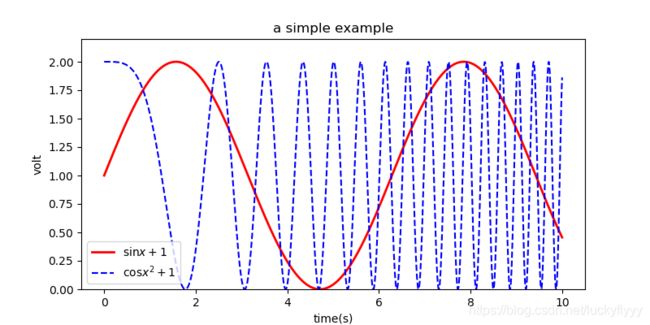
Matplotlib
# in[8]
import numpy as np
import matplotlib.pyplot as plt
x = np.linspace(0, 10, 1000)
y = np.sin(x) + 1
z = np.cos(x**2) + 1
plt.figure(figsize=(8, 4))
plt.plot(x, y, label='$\sin x+1$', color='red', linewidth=2)
plt.plot(x, z, 'b--', label=r'$\cos x^2+1$')
plt.xlabel('time(s)')
plt.ylabel('volt')
plt.title('a simple example')
plt.ylim(0, 2.2)
plt.legend()
plt.show()
Pandas
import pandas as pd
s=pd.Series([1,2,3],index=['a','b','c']) # 创建序列
d=pd.DataFrame([[1,2,3],[4,5,6]], columns = ['a','b','c']) #创建表
d2=pd.DataFrame(s) #用已有序列创建表格

d.head() #预览前面5行数据
d.describe() # 数据基本统计

# 读取文件
pd.read_excel('data.xls') #读取RXCEL文件
pd.read_csv('data.csv',encoding='utf-8')
StatsModels
# ADF平稳性检验的例子
from statsmodels.tsa.stattools import adfuller as ADF # 导入ADF验证
import numpy as np
ADF(np.random.rand(100)) # 返回的结果有ADF值和P值
Scikit_Learn
from sklearn.linear_model import LinearRegression #导入线性回归模型
model = LinearRegression() #建立线性回归模型
print(model)
Keras
Gensim
数据探索
数据质量分析
数据质量分析的主要任务是检查原始数据中是否存在脏数据,脏数据一般是指不符合要求,以及不能直接进行相应分析的数据,在常见的数据挖掘工作中,脏数据包括:缺失值,异常值,不一致值,重复数据及含有特殊符号(如#,¥,*)的数据。
- 缺失值
- 缺失值的产生的原因多种多样,主要分为机械原因和人为原因。
机械原因是由于机械原因导致的数据收集或保存的失败造成的数据缺失,比如数据存储的失败,存储器损坏,机械故障导致某段时间数据未能收集(对于定时数据采集而言)。
人为原因是由于人的主观失误、历史局限或有意隐瞒造成的数据缺失,比如,在市场调查中被访人拒绝透露相关问题的答案,或者回答的问题是无效的,数据录入人员失误漏录了数据。
- 缺失值的产生的原因多种多样,主要分为机械原因和人为原因。
- 异常值
- 异常值outlier:一组测定值中与平均值的偏差超过两倍标准差的测定值。与平均值的偏差超过三倍标准差的测定值,称为高度异常的异常值。在处理数据时,应剔除高度异常的异常值。异常值是否剔除,视具体情况而定。在统计检验时,指定为检出异常值的显著性水平α=0.05,称为检出水平;指定为检出高度异常的异常值的显著性水平α=0.01,称为舍弃水平,又称剔除水平(reject level)。
#-*- coding: utf-8 -*-
import pandas as pd

catering_sale = '../data/catering_sale.xls' #餐饮数据
data = pd.read_excel(catering_sale, index_col = u'日期') #读取数据,指定“日期”列为索引列
- 一致性
- 一致性就是数据保持一致,在分布式系统中,可以理解为多个节点中数据的值是一致的。同时,一致性也是指事务的基本特征或特性相同,其他特性或特征相类似。
数据特征分析
分布分析
分布分析能够揭示数据的分布特征和分布类型。
- 定量数据的分布分析
1) 求极差
2)决定组距,组数
3)决定分点
4)列出频率分布表
5)绘制频率分布直方图
遵循的主要原则有:
1)各组之间必须是互相排斥的
2)各组必须将所有的数据包含在内
3)各组的组宽最好相等 - 定量数据的分布分析
根据变量的类型来分组,采用饼图和条形统计图来描述分布。
# 数据统计量分析代码
from __future__ import print_function
import pandas as pd

catering_sale = '../data/catering_sale.xls' #餐饮数据
data = pd.read_excel(catering_sale, index_col = u'日期') #读取数据,指定“日期”列为索引列
data = data[(data[u'销量'] > 400)&(data[u'销量'] < 5000)] #过滤异常数据
statistics = data.describe() #保存基本统计量

statistics.loc['range'] = statistics.loc['max']-statistics.loc['min'] #极差
statistics.loc['var'] = statistics.loc['std']/statistics.loc['mean'] #变异系数
statistics.loc['dis'] = statistics.loc['75%']-statistics.loc['25%'] #四分位数间距

print(statistics)
——《python数据分析与挖掘实战》