时间序列预测——ARIMA(差分自回归移动平均模型)(1))
时间序列预测——ARIMA(差分自回归移动平均模型)
ARIMA(p,d,q)中,AR是"自回归",p为自回归项数;I为差分,d为使之成为平稳序列所做的差分次数(阶数);MA为"滑动平均",q为滑动平均项数,。ACF自相关系数能决定q的取值,PACF偏自相关系数能够决定q的取值。ARIMA原理:将非平稳时间序列转化为平稳时间序列然后将因变量仅对它的滞后值以及随机误差项的现值和滞后值进行回归所建立的模型
基本解释:
自回归模型(AR)
- 描述当前值与历史值之间的关系,用变量自身的历史时间数据对自身进行预测
- 自回归模型必须满足平稳性的要求
- 必须具有自相关性,自相关系数小于0.5则不适用
- p阶自回归过程的公式定义:
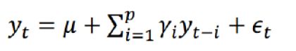
 ,y t-i 为前几天的值
PACF,偏自相关函数(决定p值),剔除了中间k-1个随机变量x(t-1)、x(t-2)、……、x(t-k+1)的干扰之后x(t-k)对x(t)影响的相关程度。
移动平均模型(MA)
- 移动平均模型关注的是自回归模型中的误差项的累加,移动平均法能有效地消除预测中的随机波动
- q阶自回归过程的公式定义:

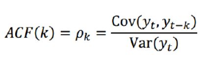
ACF,自相关函数(决定q值)反映了同一序列在不同时序的取值之间的相关性。x(t)同时还会受到中间k-1个随机变量x(t-1)、x(t-2)、……、x(t-k+1)的影响而这k-1个随机变量又都和x(t-k)具有相关关系,所 以自相关系数p(k)里实际掺杂了其他变量对x(t)与x(t-k)的影响
ARIMA(p,d,q)阶数确定:
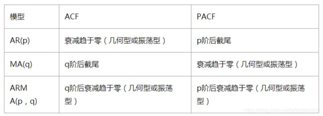
截尾:落在置信区间内(95%的点都符合该规则)
平稳性要求:平稳性就是要求经由样本时间序列所得到的拟合曲线在未来的一段期间内仍能顺着现有的形态“惯性”地延续下去
平稳性要求序列的均值和方差不发生明显变化
严平稳与弱平稳:
严平稳:严平稳表示的分布不随时间的改变而改变。
如:白噪声(正态),无论怎么取,都是期望为0,方差为1
弱平稳:期望与相关系数(依赖性)不变
未来某时刻的t的值Xt就要依赖于它的过去信息,所以需要依赖性
因为实际生活中我们拿到的数据基本都是弱平稳数据,为了保证ARIMA魔性的要求,我们需要对数据进行差分,以求数据变的平稳。
模型评估:
AIC:赤池信息准则(AkaikeInformation Criterion,AIC)
???=2?−2ln(?)
BIC:贝叶斯信息准则(Bayesian Information Criterion,BIC)
???=????−2ln(?)
k为模型参数个数,n为样本数量,L为似然函数
模型残差检验:
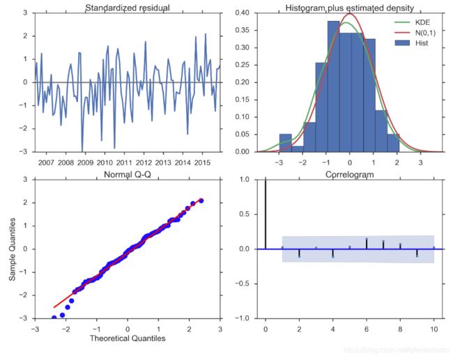
- ARIMA模型的残差是否是平均值为0且方差为常数的正态分布
- QQ图:线性即正态分布
ARIMA建模流程:
将序列平稳(差分法确定d)
p和q阶数确定:ACF与PACF
ARIMA(p,d,q)/SARIMA(p,d,q,s)呈现季节性用这个模型
%load_ext autoreload
%autoreload 2
%matplotlib inline
%config InlineBackend.figure_format='retina'

from __future__ import absolute_import, division, print_function

import sys
import os

import pandas as pd
import numpy as np

# TSA from Statsmodels
import statsmodels.api as sm
import statsmodels.formula.api as smf
import statsmodels.tsa.api as smt

# Display and Plotting
import matplotlib.pylab as plt
import seaborn as sns

pd.set_option('display.float_format', lambda x: '%.5f' % x) # pandas
np.set_printoptions(precision=5, suppress=True) # numpy

pd.set_option('display.max_columns', 100)
pd.set_option('display.max_rows', 100)

# seaborn plotting style
sns.set(style='ticks', context='poster')
filename_ts = 'data/series1.csv'
ts_df = pd.read_csv(filename_ts, index_col=0, parse_dates=[0])
n_sample = ts_df.shape[0]
print(ts_df.shape)
print(ts_df.head()) 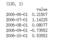
# Create a training sample and testing sample before analyzing the series

n_train=int(0.95*n_sample)+1
n_forecast=n_sample-n_train
#ts_df
ts_train = ts_df.iloc[:n_train]['value']
ts_test = ts_df.iloc[n_train:]['value']
print(ts_train.shape)
print(ts_test.shape)
print("Training Series:", "\n", ts_train.tail(), "\n")
print("Testing Series:", "\n", ts_test.head())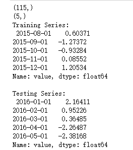
def tsplot(y, lags=None, title='', figsize=(14, 8)):
fig = plt.figure(figsize=figsize)
layout = (2, 2)
ts_ax = plt.subplot2grid(layout, (0, 0))
hist_ax = plt.subplot2grid(layout, (0, 1))
acf_ax = plt.subplot2grid(layout, (1, 0))
pacf_ax = plt.subplot2grid(layout, (1, 1))
y.plot(ax=ts_ax) # 折线图
ts_ax.set_title(title)
y.plot(ax=hist_ax, kind='hist', bins=25) #直方图
hist_ax.set_title('Histogram')
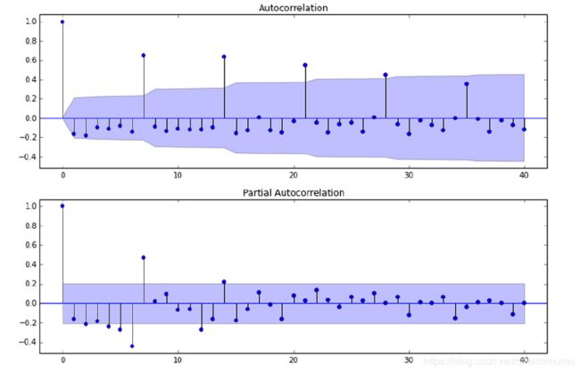
smt.graphics.plot_acf(y, lags=lags, ax=acf_ax) # ACF自相关系数
smt.graphics.plot_pacf(y, lags=lags, ax=pacf_ax) # 偏自相关系数
[ax.set_xlim(0) for ax in [acf_ax, pacf_ax]]
sns.despine()
fig.tight_layout()
return ts_ax, acf_ax, pacf_ax
tsplot(ts_train, title='A Given Training Series', lags=20); 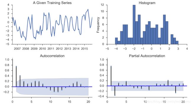
# Fit the model
arima200 = sm.tsa.SARIMAX(ts_train, order=(2,0,0)) # ARIMA季节性模型,至于p,d,q需要按照下面的方法选择
model_results = arima200.fit()
# 此处运用BIC(贝叶斯信息准则)进行模型参数选择
# 另外还可以利用AIC(赤池信息准则),视具体情况而定
import itertools
p_min = 0
d_min = 0
q_min = 0
p_max = 4
d_max = 0
q_max = 4
# Initialize a DataFrame to store the results
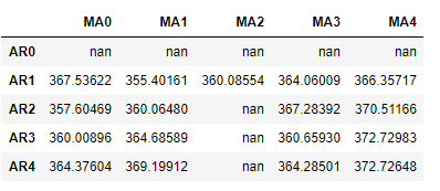
results_bic = pd.DataFrame(index=['AR{}'.format(i) for i in range(p_min,p_max+1)],
columns=['MA{}'.format(i) for i in range(q_min,q_max+1)])
for p,d,q in itertools.product(range(p_min,p_max+1),
range(d_min,d_max+1),
range(q_min,q_max+1)):
if p==0 and d==0 and q==0:
results_bic.loc['AR{}'.format(p), 'MA{}'.format(q)] = np.nan
continue
try:
model = sm.tsa.SARIMAX(ts_train, order=(p, d, q),
#enforce_stationarity=False,
#enforce_invertibility=False,
)
results = model.fit() 此处的result包含了很多信息,具体如果用到需要自己去查询
# http://www.statsmodels.org/stable/tsa.html
# print("results.bic",results.bic)
# print("results.aic",results.aic)
results_bic.loc['AR{}'.format(p), 'MA{}'.format(q)] = results.bic
except:
continue
results_bic = results_bic[results_bic.columns].astype(float)results_bic如下所示:
为了便于观察,下面对上表进行可视化:、
fig, ax = plt.subplots(figsize=(10, 8))
ax = sns.heatmap(results_bic,
                 mask=results_bic.isnull(),
                 ax=ax,
                 annot=True,
                 fmt='.2f',
                 );
ax.set_title('BIC');
//annot
//annotate的缩写,annot默认为False,当annot为True时,在heatmap中每个方格写入数据
//annot_kws,当annot为True时,可设置各个参数,包括大小,颜色,加粗,斜体字等
# annot_kws={'size':9,'weight':'bold', 'color':'blue'}
#具体查看:https://blog.csdn.net/m0_38103546/article/details/79935671 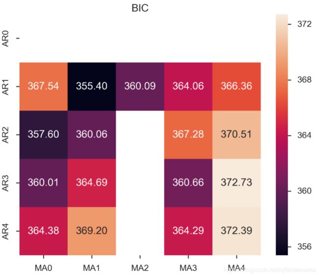
# Alternative model selection method, limited to only searching AR and MA parameters

train_results = sm.tsa.arma_order_select_ic(ts_train, ic=['aic', 'bic'], trend='nc', max_ar=4, max_ma=4)

print('AIC', train_results.aic_min_order)
print('BIC', train_results.bic_min_order)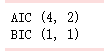
plot_diagnostics对象允许我们快速生成模型诊断并调查任何异常行为。
#残差分析 正态分布 QQ图线性

model_results.plot_diagnostics(figsize=(16, 12));
最后进行预测:
model = ARIMA(stock_train, order=(1, 1, 1),freq='W-MON')
result = model.fit()
pred = result.predict('20140609', '20160701',dynamic=True, typ='levels')
# 此处注意,2014060必须能在训练集数据中能够找到,后边的20160701则不用
print (pred)


plt.figure(figsize=(6, 6))
plt.xticks(rotation=45)
plt.plot(pred)
plt.plot(stock_train)
#预测准确性判定