方差分析
方差分析
前言
之前的预测问题都是基于量化的预测变量和响应变量,当预测变量是因子或者解释性变量的时候,回归模型无法很好的解释,此时,我们利用方差分析来解释不同组的差别(ANOVA)。这一章节涉及的软件包有gplots,car,multcomp,HH等,请自行下载。
ANOVA模型
ANOVA其实是广义线性模型的一种特殊形式,aov()函数提供的结果是比较不同组之间差异的显著性,而回归模型提供的结果是预测的值。
aov(formula,data=dataframe)
formula:Y~A+B+A:B+A*B
四种变量关系,单独的影响,交互效应,交叉影响
1.单因素方差分析
导入数据集cholesterol,治疗效果和药物每天注射量和注射次数的关系。
library(multcomp)
attach(cholesterol)
table(trt)
## trt
##  1time 2times 4times  drugD  drugE
##     10     10     10     10     10
aggregate(response,by=list(trt),FUN=mean)
##   Group.1        x
## 1   1time  5.78197
## 2  2times  9.22497
## 3  4times 12.37478
## 4   drugD 15.36117
## 5   drugE 20.94752
aggregate(response,by=list(trt),FUN=sd)
##   Group.1        x
## 1   1time 2.878113
## 2  2times 3.483054
## 3  4times 2.923119
## 4   drugD 3.454636
## 5   drugE 3.345003
fit<-aov(response~trt)
summary(fit)
##             Df Sum Sq Mean Sq F value   Pr(>F)
## trt          4 1351.4   337.8   32.43 9.82e-13 ***
## Residuals   45  468.8    10.4
## ---
## Signif. codes:  0 '***' 0.001 '**' 0.01 '*' 0.05 '.' 0.1 ' ' 1
table的结果表明每位病人都接受了每种治疗方案,aggregate的结果表明,drugE的效果最好,1times的效果最差,那么它们之间有没有明显的差异性呢?P值的结果告诉我们,差异性很显著(P<0.001)。
- 用plotmeans()来展示各组数据的均值和置信区间.
library(gplots)
plotmeans(response~trt,xlab = "Treatment",ylab="Response",main="Mean Plot with 95% CIs")
2.多重比较
ANOVA 的F检验值告诉我们各组之间存在差异性,但是并未说明具体哪两个组之间有差异性,哪两个组之间无差异性,为此,我们利用TukeyHSD()函数进行多重比较,对各组数据进行两两方差分析,得出具体结果。
TukeyHSD(fit)
##   Tukey multiple comparisons of means
##     95% family-wise confidence level
##
## Fit: aov(formula = response ~ trt)
##
## $trt
##                   diff        lwr       upr     p adj
## 2times-1time   3.44300 -0.6582817  7.544282 0.1380949
## 4times-1time   6.59281  2.4915283 10.694092 0.0003542
## drugD-1time    9.57920  5.4779183 13.680482 0.0000003
## drugE-1time   15.16555 11.0642683 19.266832 0.0000000
## 4times-2times  3.14981 -0.9514717  7.251092 0.2050382
## drugD-2times   6.13620  2.0349183 10.237482 0.0009611
## drugE-2times  11.72255  7.6212683 15.823832 0.0000000
## drugD-4times   2.98639 -1.1148917  7.087672 0.2512446
## drugE-4times   8.57274  4.4714583 12.674022 0.0000037
## drugE-drugD    5.58635  1.4850683  9.687632 0.0030633
如此,我们发现,2times-1times,4times-2times,drugD-4times之间无显著差异,其余各组之间有显著差异,将结果以图示方式表现:
par(las=2)#转动数轴标签
par(mar=c(5,8,4,2))#增加左区域
plot(TukeyHSD(fit))
- glht()函数可将模型更加形象地表现在图形上
library(multcomp)
par(mar=c(5,4,6,2))
par(las=1)
tuk<-glht(fit,linfct=mcp(trt="Tukey"))
plot(cld(tuk,level=0.05),col="lightgrey")
各组的均值一目了然,且包含了置信区间的范围。各组之间的差异性可通过对比上方字母,若两组之间不含相同字母,则存在显著性差异。由此我们得出结论,durgE的治疗方法最好,4times和drugD之间无明显差异,4times相对1times较有效,drugD相对1times和2times治疗效果更好。
3.评估检验假设
在方差分析实验中,通常假设各组数据服从正态分布,且各组方差相等。通过绘制qqplot图,我们可验证数据的正态性。
library(car)
qqPlot(lm(response~trt,data=cholesterol),simulate=T,main="Q-Q Plot",lables=F)
##qqPlot要求线性拟合几乎所有数据都落在95%置信区间内,因而正态性假设成立。
- 用bartlett检验来验证各组方差的齐性。
bartlett.test(response~trt,data=cholesterol)
##
##  Bartlett test of homogeneity of variances
##
## data:  response by trt
## Bartlett's K-squared = 0.57975, df = 4, p-value = 0.9653
结果表明各组之间的方差没有显著性差异。
4.单因素协方差分析(ANCOVA)
数据集来源于multcomp包中的litter数据:药物剂量和出生体重的关系
data(litter,package = "multcomp")
attach(litter)
table(dose)
## dose
##   0   5  50 500
##  20  19  18  17
aggregate(weight,by=list(dose),FUN=mean)
##   Group.1        x
## 1       0 32.30850
## 2       5 29.30842
## 3      50 29.86611
## 4     500 29.64647
fit2<-aov(weight~gesttime+dose)
summary(fit2)
##             Df Sum Sq Mean Sq F value  Pr(>F)
## gesttime     1  134.3  134.30   8.049 0.00597 **
## dose         3  137.1   45.71   2.739 0.04988 *
## Residuals   69 1151.3   16.69
## ---
## Signif. codes:  0 '***' 0.001 '**' 0.01 '*' 0.05 '.' 0.1 ' ' 1
ANCOVA的F检验表明:1.妊娠时间和出生重量有关联。2.药物剂量和出生重量有关联。 同样的,利用上一节的多重比较,也能找出具体哪两个组显著性差异,这里不再做演示。
- 评估模型假设 除了验证正态性和方差齐性,对于协方差分析,还应验证变量之间的交互效应,即检验回归斜率是否相同。
fit3<-aov(weight~gesttime*dose,data=litter)
summary(fit3)
##               Df Sum Sq Mean Sq F value  Pr(>F)
## gesttime       1  134.3  134.30   8.289 0.00537 **
## dose           3  137.1   45.71   2.821 0.04556 *
## gesttime:dose  3   81.9   27.29   1.684 0.17889
## Residuals     66 1069.4   16.20
## ---
## Signif. codes:  0 '***' 0.001 '**' 0.01 '*' 0.05 '.' 0.1 ' ' 1
交互性gesttime:dose 不显著,说明斜率相等,即交互效应不存在。
5.方差分析可视化
ancova()函数提供了各独立变量,协变量和因子的关系的图示。
library(HH)
ancova(weight~gesttime+dose,data=litter)
## Analysis of Variance Table
##
## Response: weight
##           Df  Sum Sq Mean Sq F value   Pr(>F)
## gesttime   1  134.30 134.304  8.0493 0.005971 **
## dose       3  137.12  45.708  2.7394 0.049883 *
## Residuals 69 1151.27  16.685
## ---
## Signif. codes:  0 '***' 0.001 '**' 0.01 '*' 0.05 '.' 0.1 ' ' 1
6.两因素方差分析
数据集为ToothGrowth,牙齿生长长度和喂食剂量,种类的关系。
attach(ToothGrowth)
table(supp,dose)
##     dose
## supp 0.5  1  2
##   OJ  10 10 10
##   VC  10 10 10
aggregate(len,by=list(supp,dose),FUN=mean)
##   Group.1 Group.2     x
## 1      OJ     0.5 13.23
## 2      VC     0.5  7.98
## 3      OJ     1.0 22.70
## 4      VC     1.0 16.77
## 5      OJ     2.0 26.06
## 6      VC     2.0 26.14
fit4<-aov(len~supp*dose)
summary(fit4)
##             Df Sum Sq Mean Sq F value   Pr(>F)
## supp         1  205.4   205.4  12.317 0.000894 ***
## dose         1 2224.3  2224.3 133.415  < 2e-16 ***
## supp:dose    1   88.9    88.9   5.333 0.024631 *
## Residuals   56  933.6    16.7
## ---
## Signif. codes:  0 '***' 0.001 '**' 0.01 '*' 0.05 '.' 0.1 ' ' 1
table函数表明各实验组数据相等,aggregate函数给出了各实验组的数据均值,aov分析表明这两种方式均有助于牙齿的生长,且相互效应也存在。
- 结果可视化
library(gplots)
interaction.plot(dose,supp,len,type="b",col=c("red","blue"),pch=c(16,18),main="Interaction between Dose and Supplement Type")
- 更具体地
library(gplots)
plotmeans(len~interaction(supp,dose,sep=" "),connect = list(c(1,3,5),c(2,4,6)),col=c("red","darkgreen"),main="Interaction Plot with 95% CIs",xlab="Treatment and Dose Combination")
分析发现,橙汁对于促进牙齿生长的效果要比维C效果好,且当剂量越大,牙齿生长越长。
- 最后,用interaction2wt()函数来生成两因素交互影响
library(HH)
interaction2wt(len~supp+dose)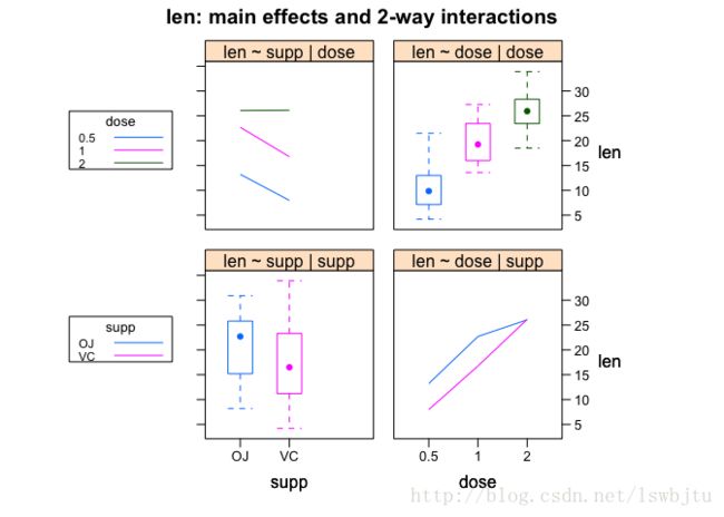
所有图形都能反映出,对于橙汁和维C,剂量增加,牙齿长度增加,对于0.5和1mg剂量,橙汁的效果比维C好。 对于这三个图形,个人认为第三种图示方法更好,它不仅展示了主要影响,还能反应交互效应的影响,图形更加具体且美观。