Record of the Task 3-5: First step to DL—— fitting, attention and CNN

第二次打卡笔记

记在前面

一点感叹

​ 因为一场比赛突如其来的变化确然是耽搁了第二次打卡的课程进程，比赛还没结束打卡又近在眼前的我在快速补课和认真琢磨清之间纠结彷徨了不少时间，还是觉得应该老老实实的动手完成一下具体的推导和实践。

​ 和助教有所交流，大约的确在基础不够的情况下直接参与这门偏向已知理论开始动手实践的我有些过于困难，但也算是有个计划在逼迫着我有所进展，不然大概的确依然会像去年一年一样浑浑噩噩的消磨过去。

​ 面对这样的压力，能做的就是尽可能在不耽误理论的情况下完成课程，同时在之后的时间主动实现代码；更好的是再去看一些理论性更深的课程，才能在这个方面更有所进展。
​
​ 也因此，这次的笔记是比较实践化的，等理论更加明确之后会继续添加补充

另

​ 因为使用的笔记软件很多快捷方式是英文字符，所以为了在听课的时候快速记录，后面内容可能会用到英文。

Task 3 过拟合/欠拟合；梯度消失/梯度爆炸；循环神经网络进阶

Fitting

​ Overfitting and underfitting are the most frequent problem in processing the NN, which comes from the discordance of the dataset, the model and the real world. Once the dataset given is largely smaller than the level of complexity of the model or the model is greatly simpler than the reality.

Solution

​ Once we met overfitting, whose culprit is the model is greatly more complex than the reality. So we can use ways like pouring to simplify the model or use ways like dropout or punish to make less connection between the neural.

• Early stop (before overfitting)
• Ensemble models (use multiple models to predict) ( 2% accuracy added )
• Regularization
  • L1/L2/Elastic punish ( make the model parameter easier )
  • Batch normalization
  • Dropout

​ Dropout has other interesting explanation about why it works.

• Ensemble models
• Break the incorporation between the cells

Gradient

​ Gradient loss comes from the gradient of the activation function by which gradient is less than 1 multiplied together caused. And Gradient explosion comes from the multiples of the weight matrix that learnt to be greater to balance the small loss.

Solution

• Ways for gradient explosion
  • Gradient clipping

• Ways for gradient loss
  • change a better activation function
  • In RNN special
    • gradient of RNN will never loss
    • to remember the chrono memory, change the way of foward

Task 4 机器翻译；注意力机制；Transformer

Sequence to Sequence

​ Encoder-Decoder is for sequence to sequence problem which is not a one-in-one-out problem, it, usually, have three types of questions. one to many: decode of generating; many to one: encode, compressing or emotion analysis; many to many but not simultaneously: translation or dialogue.

Attention

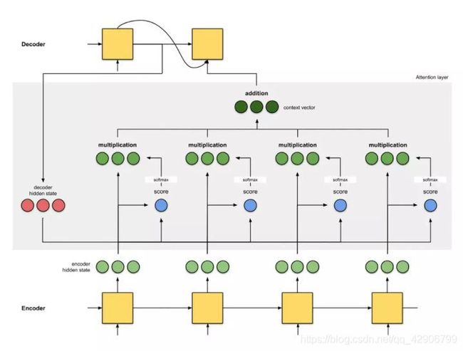
​ The problem of the seq2seq is the message will lost after a long sequence being compressed into one or several states.

​ We’ll use the attention function to give every state a score to

Task 5 卷积神经网络基础与进阶；LeNet

Convolution

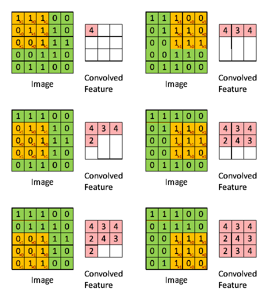
​ Convolution is a operator that is massively used in functional analysis, and also be used in the matrix operation. By using the convolution or more precisely, cross-correlation operation, which has the same result in the machine learning by using the gradient descent to learn and renew, we compress the information from the larger matrices.
​

​ With this gif from CSDN blog [1], we can visually construe the notion of convolution, and also more clearly about how it works in computer vision by compressing the details to extract the feature comes from a wider range of receptive field of the element in the smaller matrix(Activation Map’ or the ‘Feature Map‘).

we can perform operations such as Edge Detection, Sharpen and Blur just by changing the numeric values of our filter matrix before the convolution operation [8] – this means that different filters can detect different features from an image, for example edges, curves etc.

Convolution operation captures the local dependencies in the original image.

Padding and Step

​ What is the quite important part of the convolution is the padding and step which maintain the information from the edge and also control the shape of the result of convolution.

• Stride: Stride is the number of pixels by which we slide our filter matrix over the input matrix. When the stride is 1 then we move the filters one pixel at a time. When the stride is 2, then the filters jump 2 pixels at a time as we slide them around. Having a larger stride will produce smaller feature maps.

• Zero-padding: Sometimes, it is convenient to pad the input matrix with zeros around the border, so that we can apply the filter to bordering elements of our input image matrix. A nice feature of zero padding is that it allows us to control the size of the feature maps. Adding zero-padding is also called wide convolution**,** and not using zero-padding would be a narrow convolution. This has been explained clearly in [14].

About Pouring

Pouring is another way to make the image more nebulous. Spatial Pooling (also called subsampling or downsampling). It abate the calculating effort ‘reduces the number of parameters and computations in the network, therefore, controlling overfitting’ , and avoid the blur or the translation of the picture of the feature to disturb the predicting of the net.

Spatial Pooling reduces the dimensionality of each feature map but retains the most important information.

​ Then a question comes, what is the different and the similarity between pouring and convolution?

difference:

• ostentatious comprehending

  • Pouring won’t change the depth of the image.

  • Pouring don’t have specific structure parameter.

• what is the true understanding?

  • Convolution is for extracting the feature but pouring is for reducing the dimensionality.

similarity:

• We should define the size, stride, and the padding

Fully Connected Layer

The purpose of the Fully Connected layer is to use these features for classifying the input image into various classes based on the training dataset.

​ Adding a fully-connected layer is a (usually) cheap way of learning non-linear combinations of the feature.

Most of the features from convolutional and pooling layers may be good for the classification task, but combinations of those features might be even better [11].

Overall Training Process

• Step1: We initialize all filters and parameters / weights with random values

• Step2:

  The network takes a training image as input, goes through the forward propagation step (convolution, ReLU and pooling operations along with forward propagation in the Fully Connected layer) and finds the output probabilities for each class.

  • Lets say the output probabilities for the boat image above are [0.2, 0.4, 0.1, 0.3]
  • Since weights are randomly assigned for the first training example, output probabilities are also random.

• Step3:

  Calculate the total error at the output layer (summation over all 4 classes)

  • Total Error = ∑ ½ (target probability – output probability) ²

• Step4:

  Use Backpropagation to calculate the

  gradients

  of the error with respect to all weights in the network and use

  gradient descent

  to update all filter values / weights and parameter values to minimize the output error.

  • The weights are adjusted in proportion to their contribution to the total error.
  • When the same image is input again, output probabilities might now be [0.1, 0.1, 0.7, 0.1], which is closer to the target vector [0, 0, 1, 0].
  • This means that the network has learnt to classify this particular image correctly by adjusting its weights / filters such that the output error is reduced.
  • Parameters like number of filters, filter sizes, architecture of the network etc. have all been fixed before Step 1 and do not change during training process – only the values of the filter matrix and connection weights get updated.

• Step5: Repeat steps 2-4 with all images in the training set.