Kalman filter toolbox for Matlab(Matlab卡尔曼滤波工具箱)
原文地址:http://www.cs.ubc.ca/~murphyk/Software/Kalman/kalman.html
Written by Kevin Murphy, 1998.
Last updated: 7 June 2004.This toolbox supports filtering, smoothing and parameter estimation (using EM) for Linear Dynamical Systems.
- Download toolbox
- What is a Kalman filter?
- Example of Kalman filtering and smoothing for tracking
- What about non-linear and non-Gaussian systems?
- Other software for Kalman filtering, etc.
- Recommended reading
Functions
- kalman_filter
- kalman_smoother - implements the RTS equations
- learn_kalman - finds maximum likelihood estimates of the parameters using EM
- sample_lds - generate random samples
- AR_to_SS - convert Auto Regressive model of order k to State Space form
- SS_to_AR
- learn_AR - finds maximum likelihood estimates of the parameters using least squares
What is a Kalman filter?
For an excellent web site, see Welch/Bishop's KF page . For a brief intro, read on...A Linear Dynamical System is a partially observed stochastic process with linear dynamics and linear observations, both subject to Gaussian noise. It can be defined as follows, where X(t) is the hidden state at time t, and Y(t) is the observation.
   x(t+1) = F*x(t) + w(t),  w ~ N(0, Q),  x(0) ~ N(X(0), V(0))
   y(t)   = H*x(t) + v(t),  v ~ N(0, R)
The Kalman filter is an algorithm for performing filtering on this model, i.e., computing P(X(t) | Y(1), ..., Y(t)).
The Rauch-Tung-Striebel (RTS) algorithm performs fixed-interval offline smoothing, i.e., computing P(X(t) | Y(1), ..., Y(T)), for t <= T.
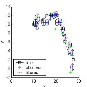
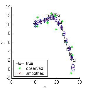
Example of Kalman filtering
Here is a simple example. Consider a particle moving in the plane at constant velocity subject to random perturbations in its trajectory. The new position (x1, x2) is the old position plus the velocity (dx1, dx2) plus noise w.[ x1(t) ] = [1 0 1 0] [ x1(t-1) ] + [ wx1 ] [ x2(t) ] [0 1 0 1] [ x2(t-1) ] [ wx2 ] [ dx1(t) ] [0 0 1 0] [ dx1(t-1) ] [ wdx1 ] [ dx2(t) ] [0 0 0 1] [ dx2(t-1) ] [ wdx2 ]We assume we only observe the position of the particle.
[ y1(t) ] =  [1 0 0 0] [ x1(t)  ] + [ vx1 ]
[ y2(t) ]    [0 1 0 0] [ x2(t)  ]   [ vx2 ]
                       [ dx1(t) ]
                       [ dx2(t) ]
Suppose we start out at position (10,10) moving to the right with velocity (1,0). We sampled a random trajectory of length 15. Below we show the filtered and smoothed trajectories.
 |
 |
What about non-linear and non-Gaussian systems?
For non-linear systems, I highly recommend the ReBEL Matlab package, which implements the extended Kalman filter, the unscented Kalman filter, etc. (See Unscented filtering and nonlinear estimation , S Julier and J Uhlmann, Proc. IEEE, 92(3), 401-422, 2004. Also, a small correction .)For systems with non-Gaussian noise, I recommend Particle filtering (PF), which is a popular sequential Monte Carlo technique. See also this discussion on pros/cons of particle filters. and the following tutorial: M. Arulampalam, S. Maskell, N. Gordon, T. Clapp, "A Tutorial on Particle Filters for Online Nonlinear/Non-Gaussian Bayesian Tracking," IEEE Transactions on Signal Processing, Volume 50, Number 2, February 2002, pp 174-189 (pdf cached here The EKF can be used as a proposal distribution for a PF. This method is better than either one alone. The Unscented Particle Filter, by R van der Merwe, A Doucet, JFG de Freitas and E Wan, May 2000.Matlab software for the UPF is also available.
Gatsby reading group on nonlinear dynamical systems