学习OpenCV范例（十四）——sobel，laplace，canny的运用

本次范例将要学习关于边缘提取，图像锐化的三个基本函数，风别是Sobel（），Laplacian（），Canny（），会从原理讲起，再到代码实现，最后会贴出运行结果，进行三种结果的对比。

1、原理及计算

Sobel：

原理：

由上图，你可以看到在 边缘 ,相素值显著的 改变 了。表示这一 改变 的一个方法是使用 导数 。 梯度值的大变预示着图像中内容的显著变化。

用更加形象的图像来解释,假设我们有一张一维图形。下图中灰度值的”跃升”表示边缘的存在:

使用一阶微分求导我们可以更加清晰的看到边缘”跃升”的存在(这里显示为高峰值)

从上例中我们可以推论检测边缘可以通过定位梯度值大于邻域的相素的方法找到(或者推广到大于一个阀值).

计算：

1. 在两个方向求导:

   1. 水平变化: 将  与一个奇数大小的内核  进行卷积。比如，当内核大小为3时,  的计算结果为:

      

   2. 垂直变化: 将I 与一个奇数大小的内核  进行卷积。比如，当内核大小为3时,  的计算结果为:

      

2. 在图像的每一点，结合以上两个结果求出近似 梯度:

   

   有时也用下面更简单公式代替:

   

注：Sobel操作，一般使用大一点的核会比小一点的核好（来自学习OpenCV），当内核大小为 3 时, 以上Sobel内核可能产生比较明显的误差(毕竟，Sobel算子只是求取了导数的近似值)。 为解决这一问题，OpenCV提供了 Scharr 函数，但该函数仅作用于大小为3的内核。该函数的运算与Sobel函数一样快，但结果却更加精确，其内核为:

Laplace：

原理：

1. Sobel算子，其基础来自于一个事实，即在边缘部分，像素值出现”跳跃“或者较大的变化。如果在此边缘部分求取一阶导数，你会看到极值的出现。正如下图所示：

   

2. 如果在边缘部分求二阶导数会出现什么情况?

   

   你会发现在一阶导数的极值位置，二阶导数为0。所以我们也可以用这个特点来作为检测图像边缘的方法。 但是， 二阶导数的0值不仅仅出现在边缘(它们也可能出现在无意义的位置),但是我们可以过滤掉这些点。

计算

Laplacian 算子 的定义:

   

内核为：

         

OpenCV函数 Laplacian 实现了Laplacian算子。 实际上，由于 Laplacian使用了图像梯度，它内部调用了 Sobel 算子。

Canny：

操作步骤：

1. 消除噪声。 使用高斯平滑滤波器卷积降噪。 下面显示了一个  的高斯内核示例:

   

2. 计算梯度幅值和方向。 此处，按照Sobel滤波器的步骤:

   1. 运用一对卷积阵列 (分别作用于  和  方向):

      

   2. 使用下列公式计算梯度幅值和方向:

      

      梯度方向近似到四个可能角度之一(一般 0, 45, 90, 135)

3. 非极大值 抑制。 这一步排除非边缘像素， 仅仅保留了一些细线条(候选边缘)。

4. 滞后阈值: 最后一步，Canny 使用了滞后阈值，滞后阈值需要两个阈值(高阈值和低阈值):

   1. 如果某一像素位置的幅值超过 高 阈值, 该像素被保留为边缘像素。
   2. 如果某一像素位置的幅值小于 低 阈值, 该像素被排除。
   3. 如果某一像素位置的幅值在两个阈值之间,该像素仅仅在连接到一个高于 高 阈值的像素时被保留。

   Canny 推荐的 高:低 阈值比在 2:1 到3:1之间。

如果想自适应确定阈值，那么请查阅这篇博客 在OpenCV中自适应确定canny算法的分割门限

2、代码实现

#include "stdafx.h"

#include "opencv2/imgproc/imgproc.hpp"
#include "opencv2/highgui/highgui.hpp"
#include 
#include 

using namespace cv;

/// 全局变量

Mat src, src_gray,grad,laplacian_dst;
Mat grad_x, grad_y,abs_grad_x, abs_grad_y,laplacian_dst1,dst, detected_edges;

int edgeThresh = 1;
int lowThreshold;
int slobel_lowThreshold;
int const max_lowThreshold = 100;
int ratio = 3;
int kernel_size = 3;
int scale = 1;
int delta = 0;
int ddepth = CV_16S;
char* window_name = "Edge Map";
char* sobel_window_name = "Sobel Demo - Simple Edge Detector";

/**
 * @函数 CannyThreshold
 * @简介： trackbar 交互回调 - Canny阈值输入比例1:3
 */
void CannyThreshold(int, void*)
{
  /// 使用 3x3内核降噪
  blur( src_gray, detected_edges, Size(3,3) );

  /// 运行Canny算子
  Canny( detected_edges, detected_edges, lowThreshold, lowThreshold*ratio, kernel_size );

  /// 使用 Canny算子输出边缘作为掩码显示原图像
  dst = Scalar::all(0);

  src.copyTo( dst, detected_edges);
  imshow( window_name, dst );
 }
void SobelThreshold(int,void*)
{
	/// 求 X方向梯度
	Sobel( src_gray, grad_x, ddepth, 1, 0, 3, scale, delta, BORDER_DEFAULT );
//	Scharr( src_gray, grad_x, ddepth, 1, 0, scale, delta, BORDER_DEFAULT );
	convertScaleAbs( grad_x, abs_grad_x );
	/// 求Y方向梯度
	Sobel( src_gray, grad_y, ddepth, 0, 1, 3, scale, delta, BORDER_DEFAULT );
//	Scharr( src_gray, grad_y, ddepth, 0, 1, scale, delta, BORDER_DEFAULT );
	convertScaleAbs( grad_y, abs_grad_y );
	/// 合并梯度(近似)
	addWeighted( abs_grad_x, 0.5, abs_grad_y, 0.5, 0, grad );
	threshold(grad,grad,slobel_lowThreshold,100,THRESH_TOZERO);
	imshow(sobel_window_name,grad);

}


/** @函数 main */
int main( int argc, char** argv )
{

  /// 装载图像
  src = imread( "lena.png");

  if( !src.data )
  { return -1; }

  /// 使用高斯滤波消除噪声
  GaussianBlur( src, src, Size(3,3), 0, 0, BORDER_DEFAULT );

  /// 创建与src同类型和大小的矩阵(dst)
  dst.create( src.size(), src.type() );

  /// 原图像转换为灰度图像
  cvtColor( src, src_gray, CV_BGR2GRAY );

  /// 创建显示窗口
  namedWindow( window_name, CV_WINDOW_AUTOSIZE );
  namedWindow(sobel_window_name,CV_WINDOW_AUTOSIZE);

  /// 创建trackbar
  createTrackbar( "Min Threshold:", window_name, &lowThreshold, max_lowThreshold, CannyThreshold );
  createTrackbar("Sobel Threshold:",sobel_window_name,&slobel_lowThreshold,max_lowThreshold, SobelThreshold);

  /// 使用Laplace函数
  Laplacian( src_gray, laplacian_dst1, ddepth, kernel_size, scale, delta, BORDER_DEFAULT );
  convertScaleAbs( laplacian_dst1, laplacian_dst );
  imshow("laplacian",laplacian_dst);

  /// 显示图像
  CannyThreshold(0, 0);
   SobelThreshold(0,0);

  /// 等待用户反应
  waitKey(0);

  return 0;
  }

3、运行结果

                                                                         图1、 原图

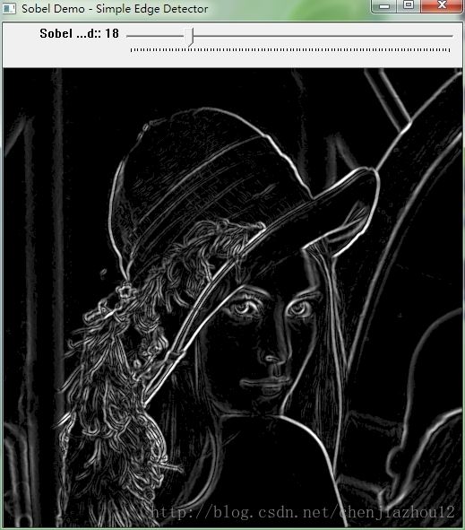
                                                            图2、Sobel

                                                                图3、scharr

                                                            图4、laplace

                                                                   图5、canny

4、使用的类和函数

Sobel：

功能：使用扩展 Sobel 算子计算一阶、二阶、三阶或混合图像差分

结构：

void Sobel(InputArray src, OutputArray dst, int ddepth, int xorder, int yorder, int ksize=3, double scale=1, double delta=0, int borderType=BORDER_DEFAULT )

src ：源图像
dst ：目标图像，和源图像有同样的size和通道数
ddepth ：目标图像的深度
xorder ：x 方向上的差分阶数
yorder ：y 方向上的差分阶数
ksize ：扩展 Sobel 核的大小，必须是 1, 3, 5 或 7
scale ：缩放因子
delta ：最后加到图像中的数值
borderType ：边界插值类型

通过适当的核对图像进行卷积：

如果ksize=3，x方向的核为：

y方向的核为：

Laplacian：

功能：计算图像的 Laplacian 变换

结构：

void Laplacian(InputArray src, OutputArray dst, int ddepth, int ksize=1, double scale=1, double delta=0, int borderType=BORDER_DEFAULT )

src ：源图像
dst ：目标图像，和源图像有同样的size和通道数
ddepth ：目标图像的深度
ksize ：核的大小，必须为奇数
scale ：缩放因子
delta ：最后加到图像中的数值
borderType ：边界插值类型
函数 Laplacian 计算输入图像的 Laplacian变换，方法是先用 sobel 算子计算二阶 x- 和 y- 差分，再求和:

对 ksize=1 则给出最快计算结果，相当于对图像采用如下内核做卷积：

Canny：

功能：采用 Canny 算法做边缘检测

结构：

void Canny(InputArray image, OutputArray edges, double threshold1, double threshold2, int apertureSize=3, bool L2gradient=false )

image ：单通道8位图像
edges：目标图像，和源图像有同样的size和type
threshold1 ：第一个阈值
threshold2 ：第二个阈值
apertureSize ：sobel内核大小
L2gradient ：当L2gradient=true，则梯度幅度采用L_2范式计算 ，当为false时，使用L_1范式

函数 Canny 采用 CANNY 算法发现输入图像的边缘而且在输出图像中标识这些边缘。threshold1和threshold2 当中的小阈值用来控制边缘连接，大的阈值用来控制强边缘的初始分割。

注意：Canny只接受单通道图像作为输入。