Event-B建模实际操作：控制桥上的汽车（四）

接上节；在这一次精化中，我们将引入传感器，这是一种能够检查汽车上桥或下桥的物理情况的设备。

 

Third Refinement: Introducing Car Sensors

In this refinement, we introduce the sensors, which are devices capable of detecting the physical presence of cars entering or leaving the bridge. We remind the reader that such sensors are situated on each side of the road and at both extremities of the bridge. This is indicated in Fig. 58.

Fig. 58. The Bridge Control Equipment

 

Closed Model of the Controller and its Environment. The presence of the sensor must now make clearer the separation between our future software controller and its physical environment. This can be sketched as indicated in the diagram of Fig. 59.

Fig. 59. Controller and Environment

 

As can be seen, the software controller is equipped with two sets of channels: output channels connecting the controller to the traffic lights and input channels connecting the sensors to the software controller. Our intention is to build now a closed model corresponding to a complete mathematical simulation of the pair formed by the software controller and its environment. The reason for building such a model is that we want to be sure that the controller works in perfect harmony with the environment, provided, of course, the latter obeys a number of assumptions that have to be made completely clear.

In Rodin, firstly we need to create a new Context. Use File à New à Event-B Component or right-click on the newly created project and select New à Event-B Component. Use SENSOR as the component name, select Context as component-type, and click Finish. Then, add a carrier set and two constants into the context SENSOR.

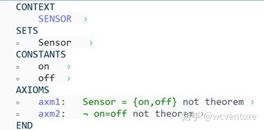
We must extend our set of constants by introducing the set Sensor and its two distinct values on and off. And we can also claim that Sensor = {on, off} and on ≠ off. The built context can be seen as Fig. 60.

Fig. 60. Context SENSOR

 

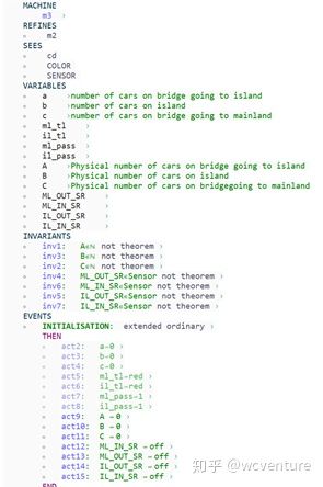
Then create a refinement is by right-clicking on the machine m2 in the project browser and selecting Refine. This will create a “stub” consisting of all variables and events. Here I create a machine with the name m3. After creating the machine file. We need to add the relationship between machine file and context file and connect machine file m3 to context file cd. We know that the environment is formalized by means of four variables corresponding to the state of the sensors. More precisely, a sensor can be in one of two states: either "on" or "off". It is "on" when a car is on it, "off" otherwise. As a consequence, we shall enlarge our state with four variables corresponding to each sensor state: ML_OUT_SR, ML_IN_SR, IL_OUT_SR, and IL_IN_SR. Notice that we use upper case letters to name these variables, this is to remember that they are physical variables denoting objects of the real world. We shall also introduce three variables A, B, and C denoting the physical number of cars on the bridge going to the island (A), on the island (B), and on the bridge going to the mainland (C). After adding new variables, the machine is shown in Fig. 61.

 

Fig. 61. Adding Sensor in Machine m3

It remains now for us to explain how the sensors communicate with the controller. We are not interested in the precise technology used in the sensors, only in their external behavior. As said above, a sensor can be in two different states: either "on" or "off". When the state of a sensor moves from "off" to"on", it means that a car has just been detected as arriving on it: nothing has to be sent to the controller in this case. Note that the state of a sensor can remain "on" for a certain time when the car has to wait because the associated traffic light is red. When the state of a sensor moves from "on" to"off", it means that a car, which was on it, has just left it. In that case, a message has to be sent to the controller. All this is illustrated in the diagram of Fig. 62

Fig. 62. Controller and Environment

We thus introduce four input channel variables corresponding to the different sensors: ml_out_10, ml_in_10, il_in_10, and il_out_10. After adding new variables, the machine is shown in Fig. 63.

Fig. 63. Adding ml_out_10, ml_in_10, il_in_10, and il_out_10 in Machine m3

Understanding: The diagram of Fig. 64 shows the various categories of variables of our closed system. In principle, the input channel variables are set by the environment and tested by the controller. Likewise, the output channel variables are set by the controller and tested by the environment. On the other hand, the controller variables are set and tested by the controller only while the environment variables are set and tested by the environment only. There is no exception to these rules.

Fig. 64. Controller, Environment, and their Variables

We are now going to state the more interesting invariants concerned with these variables. First, we have an invariant stating that when the sensor IL_IN_SR is on, then A is positive. In other words, there is at least one physical car on the bridge, namely the one that sits on the sensor IL_IN_SR. We have similar invariants for IL_OUT_SR and ML_IN_SR, yielding:

 

Second, when input channel ml_out_10 is TRUE, it means that a car has just left the sensorML_OUT_SR. For this to be possible the mainland traffic light must be green. This invariant formalizes the fact that car drivers obey the traffic light indications. We have a similar case with input channel il_out_10. This is formalized by means of the following two invariants:

Our next group of invariants is dealing with the relationship between the sensor status and the messages sent to the controller. They say that no message is on an input channel when a car is on the corresponding sensor. Here are these invariants:

These invariants state that when a car is on a sensor then the previous message coming from that sensor has been treated by the controller. In fact, it corresponds to a requirement which is obviously missing in our requirement document:

FUN-5: The controller must be fast enough so as to be able to treat all the information coming from the environment.

Our next series of invariants is dealing with the relationship that exists between the physical number of cars (A, B, and C) and the corresponding numbers dealt with by the controller (a, b, and c). These invariants are easy to understand. When, say, il_in_10 = TRUE, it means that a car has left the bridge to enter the island, but the controller does not know it yet: thus, A is incremented and B is decremented while a and b are left unchanged. Likewise, when ml_out_10 = TRUE, it means that a new car has entered the bridge coming from the mainland, but the controller does not know it yet: thus, A is incremented while a is left unchanged. We have similar invariants dealing with B and b and with C and c as shown in Fig. 65.

Fig. 65. The connection between physical and logical numbers

The last two, and probably most important, invariants in this refinement are the ones which say that the two main properties (one-way bridge and the limited number of cars) hold for the physical number of cars, as shown in Fig. 58. In other words, the controller although working with slightly time-shifted information concerning A, B, and C (the controller bases its decision on a, b, and c), nevertheless maintains the basic properties on the physical numbers of cars A, B, and C.

Fig. 66. Law of physical variables

However, now we cannot prove all the proof Obligation, as we need to check each event and refine it.

Fig. 67. Proof Obligation of ML_out1 and ML_out2

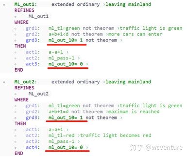
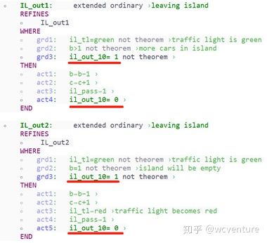
It is now easy to proceed with the refinement of abstract events. This is done in a straightforward fashion as shown in Fig. 68, Fig. 69, and Fig. 70. Notice that in their abstract versions these events were testing the green status of the corresponding traffic lights. In these refined versions, it is not necessary anymore since these events are now triggered by the input channels ml_out_10 or il_out_10 which ensure through invariants inv15 and inv16 that the corresponding lights are green.

Fig. 68. Refined ML_out1 and ML_out2

Fig. 69. Refined IL_out1 and IL_out2

Fig. 70. Refined ML_in and IL_in

 

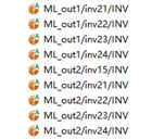
After refining abstract events, some proof obligation can be automatically discharged, as shown in Fig. 71.

Fig. 71. Proof Obligation of ML_out1 and ML_out2

However, ML_tl_green/inv16 and IL_tl_green/inv15/INV cannot be discharged.

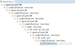
Form the proof Tree of ML_tl_green/inv16/INV, we can see that we need to proof il_out≠1, as shown in Fig. 72.

Fig. 72. The Proof Tree of ML_tl_green/inv16/INV

The new guard il_out_10 = 0 in event ML_tl_green is indispensable to maintain invariant inv16. This is so because il_tl is set to red in event ML_tl_green. We have a similar guard (ml_out_10 = 0) in event IL_tl_green: it is necessary in order to maintain invariant inv15. The refined ML_tl_green and IL_tl_green can be seen in Fig. 73.

Fig. 73. The Refined Event ML_tl_green and IL_tl_green

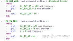
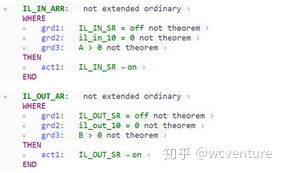
We still need to add new events to the Environment. We add four new events corresponding to cars arriving on the various sensors, as shown in Fig. 7466. In each case, we suppose that the previous message has been treated: the input channels are all tested for FALSE. Moreover, the physical number of cars is tested as expected. It expresses the fact that the setting to "on" of a sensor is due to the presence of cars. This is compatible with our requirement ENV-5 saying that the sensors are used to detect the presence of a car entering or leaving the bridge.

Fig. 74. Four new events corresponding to cars arriving on the various sensors

 

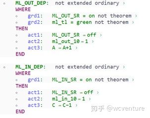
We also have four events corresponding to a car leaving a sensor, as shown in Fig. 75. It is important to notice that a car leaving the mainland out-sensor can do so provided the corresponding traffic light is green. Likewise, a car leaving the island out-sensor can do so provided the corresponding traffic light is green. Here we take into account requirement ENV-3 saying that "cars are not supposed to pass on a red traffic light, only on a green one". It is also possible to see that in each case a message is sent to the controller. Finally, the physical number of cars are modified as expected: we simulate what happens in the environment.

Fig. 75. Four new events corresponding to a car leaving a sensor

 

We have to exhibit a variant which is decreased by all new events.

Here it is the variant:

12−(ML_OUT_SR+ML_IN_SR+IL_OUT_SR+IL_IN_SR+2∗(il_out_10+ml_out_10+ml_in_10+il_in_10))

We finally need to prove that this third refinement does not deadlock.

As a whole, the second refined model (context + machine) design by Rodin is shown as follows.

Context SENSOR (final version):

CONTEXT

SENSOR ›

SETS

⚬ Sensor ›

CONSTANTS

⚬ on ›

⚬ off ›

AXIOMS

⚬ axm1: Sensor = {on,off} not theorem ›

⚬ axm2: ¬ on=off not theorem ›

END

Machine m3 (final version):

MACHINE

m3 ›

REFINES

⚬ m2

SEES

⚬ cd

⚬ COLOR

⚬ SENSOR

VARIABLES

⚬ a ›as in previous abstraction

⚬ b ›as in previous abstraction

⚬ c ›as in previous abstraction

⚬ ml_tl ›as in previous abstraction

⚬ il_tl ›as in previous abstraction

⚬ il_pass ›as in previous abstraction

⚬ ml_pass ›as in previous abstraction

⚬ A ›Physical number of cars on bridge going to island

⚬ B ›Physical number of cars on island

⚬ C ›Physical number of cars on bridgegoing to mainland

⚬ ML_OUT_SR ›sensor

⚬ ML_IN_SR ›sensor

⚬ IL_OUT_SR ›sensor

⚬ IL_IN_SR ›sensor

⚬ ml_out_10 ›wire from sensor to controller

⚬ il_out_10 ›wire from sensor to controller

⚬ ml_in_10 ›wire from sensor to controller

⚬ il_in_10 ›wire from sensor to controller

INVARIANTS

⚬ inv1: IL_IN_SR = on ⇒ A>0 not theorem ›car on sensor means there is a car

⚬ inv2: IL_OUT_SR = on ⇒ B>0 not theorem ›car on sensor means there is a ca

⚬ inv3: ML_IN_SR = on ⇒ C>0 not theorem ›car on sensor means there is a ca

⚬ inv4: ml_out_10 = TRUE ⇒ ml_tl=green not theorem ›A car passed, the traffic light must have been green

⚬ inv5: il_out_10 = TRUE ⇒ il_tl = green not theorem ›A car passed, the traffic light must have been green

⚬ inv6: IL_IN_SR = on ⇒ il_in_10 = FALSE not theorem ›

⚬ inv7: IL_OUT_SR = on ⇒ il_out_10 = FALSE not theorem ›

⚬ inv8: ML_IN_SR = on ⇒ ml_in_10 = FALSE not theorem ›

⚬ inv9: ML_OUT_SR = on ⇒ ml_out_10 = FALSE not theorem ›

⚬ inv10: il_in_10 = TRUE ∧ ml_out_10 = TRUE ⇒ A = a not theorem ›Connection between physical and logical numbers

⚬ inv11: il_in_10 = FALSE ∧ ml_out_10 = TRUE ⇒ A = a+1 not theorem ›

⚬ inv12: il_in_10 = TRUE ∧ ml_out_10 = FALSE ⇒ A = a−1 not theorem ›

⚬ inv13: il_in_10 = FALSE ∧ ml_out_10 = FALSE ⇒ A = a not theorem ›

⚬ inv14: il_in_10 = TRUE ∧ il_out_10 = TRUE ⇒ B=b not theorem ›

⚬ inv15: il_in_10 = TRUE ∧ il_out_10 = FALSE ⇒ B = b+1 not theorem ›

⚬ inv16: il_in_10 = FALSE ∧ il_out_10 = TRUE ⇒ B = b−1 not theorem ›

⚬ inv17: il_in_10 = FALSE ∧ il_out_10 = FALSE ⇒ B=b not theorem ›

⚬ inv18: il_out_10 = TRUE ∧ ml_in_10 = TRUE ⇒ C=c not theorem ›

⚬ inv19: il_out_10 = TRUE ∧ ml_in_10 = FALSE ⇒ C=c+1 not theorem ›

⚬ inv20: il_out_10 = FALSE ∧ ml_in_10 = TRUE ⇒ C=c−1 not theorem ›

⚬ inv21: il_out_10 =FALSE ∧ ml_in_10 = FALSE ⇒ C=c not theorem ›

⚬ inv22: A=0 ∨ C=0 not theorem ›Law of physical variables

⚬ inv23: A+B+C ≤ d not theorem ›Law of physical variables

⚬ inv24: A∈ℕ not theorem ›

⚬ inv25: B∈ℕ not theorem ›

⚬ inv26: C∈ℕ not theorem ›

EVENTS

⚬ INITIALISATION: not extended ordinary ›

THEN

⚬ act2: a ≔ 0 ›

⚬ act3: b ≔ 0 ›

⚬ act4: c ≔ 0 ›

⚬ act1: ml_tl≔red ›

⚬ act5: il_tl≔red ›

⚬ act6: ml_pass≔1 ›

⚬ act7: il_pass≔1 ›

⚬ act15: ml_out_10 ≔ FALSE ›

⚬ qct16: il_out_10 ≔ FALSE ›

⚬ act17: ml_in_10 ≔ FALSE ›

⚬ act18: il_in_10 ≔ FALSE ›

⚬ act8: A ≔ 0 ›

⚬ act9: B ≔ 0 ›

⚬ act10: C ≔ 0 ›

⚬ act11: ML_IN_SR ≔ off ›

⚬ act12: ML_OUT_SR ≔ off ›

⚬ act13: IL_OUT_SR ≔ off ›

⚬ act14: IL_IN_SR ≔ off ›

END

⚬ ML_out1: not extended ordinary ›

REFINES

⚬ ML_out1

WHERE

⚬ grd1: ml_out_10= TRUE not theorem ›

⚬ grd2: a+b+1

THEN

⚬ act1: a≔a+1 ›

⚬ act2: ml_pass≔1 ›

⚬ act3: ml_out_10 ≔ FALSE ›

END

⚬ ML_out2: not extended ordinary ›

REFINES

⚬ ML_out2

WHERE

⚬ grd1: ml_out_10 = TRUE not theorem ›

⚬ grd2: a+b+1=d not theorem ›

THEN

⚬ act1: a≔a+1 ›

⚬ act2: ml_tl≔red ›

⚬ act3: ml_pass≔1 ›

⚬ act4: ml_out_10 ≔ FALSE ›

END

⚬ IL_out1: not extended ordinary ›

REFINES

⚬ IL_out1

WHERE

⚬ grd1: il_out_10 = TRUE not theorem ›

⚬ grd2: b>1 not theorem ›

THEN

⚬ act1: b≔b−1 ›

⚬ act2: c≔c+1 ›

⚬ act3: il_pass≔1 ›

⚬ act4: il_out_10 ≔ FALSE ›

END

⚬ IL_out2: not extended ordinary ›

REFINES

⚬ IL_out2

WHERE

⚬ grd1: il_out_10 = TRUE not theorem ›

⚬ grd2: b=1 not theorem ›

THEN

⚬ act1: b≔b−1 ›

⚬ act2: il_tl≔red ›

⚬ act3: c≔c+1 ›

⚬ act4: il_pass≔1 ›

⚬ act5: il_out_10 ≔ FALSE ›

END

⚬ ML_tl_green: not extended convergent ›

REFINES

⚬ ML_tl_green

WHERE

⚬ grd1: ml_tl=red not theorem ›

⚬ grd2: a+b

⚬ grd3: c=0 not theorem ›

⚬ grd4: il_pass=1 not theorem ›

⚬ grd5: il_out_10 = FALSE not theorem ›

⚬ grd6: ML_OUT_SR = on not theorem ›

THEN

⚬ act1: ml_tl≔green ›

⚬ act2: il_tl≔red ›

⚬ act3: ml_pass≔0 ›

END

⚬ IL_tl_green: not extended convergent ›

REFINES

⚬ IL_tl_green

WHERE

⚬ grd1: il_tl=red not theorem ›

⚬ grd2: 0

⚬ grd3: a=0 not theorem ›

⚬ grd4: ml_pass=1 not theorem ›

⚬ grd5: ml_out_10 = FALSE not theorem ›

⚬ grd6: IL_OUT_SR = on not theorem ›

THEN

⚬ act1: il_tl≔green ›

⚬ act2: ml_tl≔red ›

⚬ act3: il_pass≔0 ›

END

⚬ ML_in: not extended ordinary ›

REFINES

⚬ ML_in

WHERE

⚬ grd1: ml_in_10 = TRUE not theorem ›

⚬ grd2: c>0 not theorem ›

THEN

⚬ act1: c ≔ c−1 ›

⚬ act2: ml_in_10 ≔ FALSE ›

END

⚬ IL_in: not extended ordinary ›

REFINES

⚬ IL_in

WHERE

⚬ grd1: il_in_10 = TRUE not theorem ›

⚬ grd2: 0 < a not theorem ›

THEN

⚬ act1: a ≔ a−1 ›

⚬ act2: b ≔ b+1 ›

⚬ act3: il_in_10 ≔ FALSE ›

END

⚬ ML_OUT_ARR: not extended ordinary ›Physical Events

WHERE

⚬ grd1: ML_OUT_SR = off not theorem ›

⚬ grd2: ml_out_10 = FALSE not theorem ›

THEN

⚬ act1: ML_OUT_SR ≔ on ›

END

⚬ ML_IN_ARR: not extended ordinary ›

WHERE

⚬ grd1: ML_IN_SR = off not theorem ›

⚬ grd2: ml_in_10 = FALSE not theorem ›

⚬ grd3: C > 0 not theorem ›

THEN

⚬ act1: ML_IN_SR ≔ on ›

END

⚬ IL_IN_ARR: not extended ordinary ›

WHERE

⚬ grd1: IL_IN_SR = off not theorem ›

⚬ grd2: il_in_10 = FALSE not theorem ›

⚬ grd3: A > 0 not theorem ›

THEN

⚬ act1: IL_IN_SR ≔ on ›

END

⚬ IL_OUT_AR: not extended ordinary ›

WHERE

⚬ grd1: IL_OUT_SR = off not theorem ›

⚬ grd2: il_out_10 = FALSE not theorem ›

⚬ grd3: B > 0 not theorem ›

THEN

⚬ act1: IL_OUT_SR ≔ on ›

END

⚬ ML_OUT_DEP: not extended ordinary ›

WHERE

⚬ grd1: ML_OUT_SR = on not theorem ›

⚬ grd2: ml_tl = green not theorem ›

THEN

⚬ act1: ML_OUT_SR ≔ off ›

⚬ act2: ml_out_10 ≔ TRUE ›

⚬ act3: A ≔ A+1 ›

END

⚬ ML_IN_DEP: not extended ordinary ›

WHERE

⚬ grd1: ML_IN_SR = on not theorem ›

THEN

⚬ act1: ML_IN_SR ≔ off ›

⚬ act2: ml_in_10 ≔ TRUE ›

⚬ act3: C ≔ C−1 ›

END

⚬ IL_IN_DEP: not extended ordinary ›

WHERE

⚬ grd1: IL_IN_SR = on not theorem ›

THEN

⚬ act1: IL_IN_SR ≔ off ›

⚬ act2: il_in_10 ≔ TRUE ›

⚬ act3: A ≔ A−1 ›

⚬ act4: B ≔ B+1 ›

END

⚬ IL_OUT_DEP: not extended ordinary ›

WHERE

⚬ grd1: IL_OUT_SR = on not theorem ›

⚬ grd2: il_tl = green not theorem ›

THEN

⚬ act1: IL_OUT_SR ≔ off ›

⚬ act2: il_out_10 ≔ TRUE ›

⚬ act3: B ≔ B−1 ›

⚬ act4: C ≔ C+1 ›

END

END