医学统计分析思路方法总结：实例

医学研究思路

研究适合的研究数据

模型选择

• 分类变量：logistic回归
• 生存资料 Cox回归
• 计数资料：Poisson/负二项
• 回归连续变量：线性回归

选择适合的预测分子

• 阅读文献选择适当的预测因子

临床医学预测模型的流程

R数据导入和查看和导出

• 

结局变量==Y值

二分类

• 诊断模型中转化为二分类模型

  • 诊断模型中结局变量的形式:
  • 二分类:是否患病
  • 由连续变量根据某一标准转换为二分类:是否高血压
  • 连续变量:血压值
    • 对于诊断模型，如果结局变量是连续变量，需要考虑是否要转换为二分类变量。

• 

连续变量

• • 

rm(list = ls())


# install and load packages

install.packages("pROC")
install.packages("maxstat")
install.packages("survminer")
install.packages("survival")
install.packages("rms")

library(pROC)
library(maxstat)
library(survminer)
library(survival)
library(rms)

# read data
data_exercise <- read.csv('data_exercise.csv')

data <- data_exercise

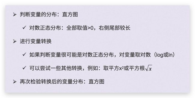
## 1. variable transformation based on distribution

# 1.1 check distribution
hist_outlier(data$C1) # normal

hist_outlier(data$C6) # log-normal

hist_outlier(data$C5) # ??


# 1.2 try transformations
data$C6_log <- log(data$C6) #log

data$C5_log_minus <- log(max(data$C5)+1-(data$C5))

# 1.3 check distribution after transformation
hist_outlier(data$C6_log)

hist_outlier(data$C5_log_minus)



## 2. variable transformation based on relation Y~X


# 2.1 categorize continuous variable to categorical variable based on pre-defined cut-offs

data$X_group<-cut(data$X, c(-1000,36,38,1000), labels=c("low","normal","high"))


# 2.2 use splines (rcs) to explore relation Y~x

# create a new variable D1 (with a U-shape relation)

data$D1 <- -data$C4
data$D1 <- ifelse(data$D1<0,data$D1,data$C3)


dd <- datadist(data)
options(datadist="dd")


fit.C3 <- cph(Surv(Time_death, Status_death==1)~ rcs(C3,3),data=data)
plot(Predict(fit.C3,C3,ref.zero=TRUE))


fit.C4 <- cph(Surv(Time_death, Status_death==1)~ rcs(C4,3),data=data)
plot(Predict(fit.C4,C4,ref.zero=TRUE))
              

fit.C5 <- cph(Surv(Time_death, Status_death==1)~ rcs(C5,3),data=data)
plot(Predict(fit.C5,C5,ref.zero=TRUE))


fit.D1.cox <- cph(Surv(Time_death, Status_death==1)~ rcs(D1,3),data=data)
plot(Predict(fit.D1.cox,D1,ref.zero=TRUE))


# change the reference value to 0

dd$limits$D1[2] <- 0
options(datadist="dd")

fit.D1.cox <- cph(Surv(Time_death, Status_death==1)~ rcs(D1,3),data=data)
plot(Predict(fit.D1.cox,D1,ref.zero=TRUE))


# also applies to logistic regression

fit.D1.logistic <- lrm(Status_death ~ rcs(D1,3),data=data,x=TRUE,y=TRUE)
plot(Predict(fit.D1.logistic,D1,ref.zero=TRUE))


# also applies to ggplot

ggplot(Predict(fit.D1.cox,D1,ref.zero=TRUE))



# 2.3 Transformation U-shape

data$D1_sq <- (data$D1-(-0.1))^2

dd <- datadist(data)
options(datadist="dd")


fit.D1_sq.cox <- cph(Surv(Time_death, Status_death==1)~ rcs(D1_sq,3),data=data)
plot(Predict(fit.D1_sq.cox,D1_sq,ref.zero=TRUE))



# 2.4 categorize continuous variable to categorical variable based on shapes


plot(Predict(fit.D1.cox,D1,ref.zero=TRUE))



data$D1_group<-cut(data$D1, c(-1000,-0.5,0.5,1000), labels=c("low","normal","high"))


fit.D1_group.cox <- coxph(Surv(Time_death, Status_death==1)~ relevel(D1_group,ref="normal"),data=data)

summary(fit.D1_group.cox)

异常值处理

错误值

• [外链图片转存失败,源站可能有防盗链机制,建议将图片保存下来直接上传(img-BthiFgW0-1594014200622)(https://i.loli.net/2020/06/30/NaXg6ycukZos3xS.png)]
• [外链图片转存失败,源站可能有防盗链机制,建议将图片保存下来直接上传(img-pDo2BfuR-1594014200623)(https://i.loli.net/2020/06/30/wFa579zGU3fHLig.png)]

异常值

• [外链图片转存失败,源站可能有防盗链机制,建议将图片保存下来直接上传(img-aWU3Li5q-1594014200624)(https://i.loli.net/2020/06/30/qkZOv8p3M4GA7jw.png)]
• 处理方法
  • [外链图片转存失败,源站可能有防盗链机制,建议将图片保存下来直接上传(img-8d5E634x-1594014200624)(https://i.loli.net/2020/06/30/WrjIqXxY8FL7cMe.png)]

缺失值