基于简单神经网络模型的鸢尾花分类问题
摘要
本人在学习《Python机器学习基础教程》时的一些小实验。
一、认识鸢尾花数据
python的机器学习库scikit-learn中保存了大量的经典的实验数据集,在学习阶段没有办法搜集大数据的情况下,可以用这些数据进行学习。
首先从sklearn.datasets中导入鸢尾花(iris)的数据集
from sklearn.datasets import load_iris
iris = load_iris()
对象iris是一个Bunch对象,与字典很类似,可以用iris.keys()查看所有键。这里只介绍需要用得到的键
print(iris['DESCR'], '\n') #鸢尾花数据集的摘要
print("The target name of iris: {}".format(iris['target_names'])) #标签名字
print("The target by number: \n{}".format(iris['target'])) #标签
.. _iris_dataset:

Iris plants dataset
--------------------

**Data Set Characteristics:**

    :Number of Instances: 150 (50 in each of three classes)
    :Number of Attributes: 4 numeric, predictive attributes and the class
    :Attribute Information:
        - sepal length in cm
        - sepal width in cm
        - petal length in cm
        - petal width in cm
        - class:
                - Iris-Setosa
                - Iris-Versicolour
                - Iris-Virginica

    :Summary Statistics:

    ============== ==== ==== ======= ===== ====================
                    Min  Max   Mean    SD   Class Correlation
    ============== ==== ==== ======= ===== ====================
    sepal length:   4.3  7.9   5.84   0.83    0.7826
    sepal width:    2.0  4.4   3.05   0.43   -0.4194
    petal length:   1.0  6.9   3.76   1.76    0.9490  (high!)
    petal width:    0.1  2.5   1.20   0.76    0.9565  (high!)
    ============== ==== ==== ======= ===== ====================

    :Missing Attribute Values: None
    :Class Distribution: 33.3% for each of 3 classes.
    :Creator: R.A. Fisher
    :Donor: Michael Marshall (MARSHALL%PLU@io.arc.nasa.gov)
    :Date: July, 1988

The famous Iris database, first used by Sir R.A. Fisher. The dataset is taken
from Fisher's paper. Note that it's the same as in R, but not as in the UCI
Machine Learning Repository, which has two wrong data points.

This is perhaps the best known database to be found in the
pattern recognition literature.  Fisher's paper is a classic in the field and
is referenced frequently to this day.  (See Duda & Hart, for example.)  The
data set contains 3 classes of 50 instances each, where each class refers to a
type of iris plant.  One class is linearly separable from the other 2; the
latter are NOT linearly separable from each other.

.. topic:: References

   - Fisher, R.A. "The use of multiple measurements in taxonomic problems"
     Annual Eugenics, 7, Part II, 179-188 (1936); also in "Contributions to
     Mathematical Statistics" (John Wiley, NY, 1950).
   - Duda, R.O., & Hart, P.E. (1973) Pattern Classification and Scene Analysis.
     (Q327.D83) John Wiley & Sons.  ISBN 0-471-22361-1.  See page 218.
   - Dasarathy, B.V. (1980) "Nosing Around the Neighborhood: A New System
     Structure and Classification Rule for Recognition in Partially Exposed
     Environments".  IEEE Transactions on Pattern Analysis and Machine
     Intelligence, Vol. PAMI-2, No. 1, 67-71.
   - Gates, G.W. (1972) "The Reduced Nearest Neighbor Rule".  IEEE Transactions
     on Information Theory, May 1972, 431-433.
   - See also: 1988 MLC Proceedings, 54-64.  Cheeseman et al"s AUTOCLASS II
     conceptual clustering system finds 3 classes in the data.
   - Many, many more ...

The target name of iris: ['setosa' 'versicolor' 'virginica']
The target by number:
[0 0 0 0 0 0 0 0 0 0 0 0 0 0 0 0 0 0 0 0 0 0 0 0 0 0 0 0 0 0 0 0 0 0 0 0 0
 0 0 0 0 0 0 0 0 0 0 0 0 0 1 1 1 1 1 1 1 1 1 1 1 1 1 1 1 1 1 1 1 1 1 1 1 1
 1 1 1 1 1 1 1 1 1 1 1 1 1 1 1 1 1 1 1 1 1 1 1 1 1 1 2 2 2 2 2 2 2 2 2 2 2
 2 2 2 2 2 2 2 2 2 2 2 2 2 2 2 2 2 2 2 2 2 2 2 2 2 2 2 2 2 2 2 2 2 2 2 2 2
 2 2]
说明:
feature_name是特征名,一共有四种,分别代表花萼长,花萼宽,花瓣长,花瓣宽
:Attribute Information:
        - sepal length in cm
        - sepal width in cm
        - petal length in cm
        - petal width in cm
target_name是标签(类别)名,一共分为三类
- Class:
           - Iris-Setosa
           - Iris-Versicolour
           - Iris-Virginica
target是标签的代号,如下
{

	'Iris-Setosa':0,
 	'Iris-Versicolour':1,
 	'Iris-Virginica':2
 	}
data是鸢尾花的样本数据集,一共有150个样本点,每个样本点提供了4个特征和分类的数据.
我们用pandas的DataFrame来展现数据集(限于篇幅只展示部分)
import pandas as pd
from IPython.display import display

data = {
     'sl':iris['data'][:,0],
        'sw':iris['data'][:,1],
        'pl':iris['data'][:,2],
        'pw':iris['data'][:,3],
        'target':iris['target']}
data_pandas = pd.DataFrame(data)

display(data_pandas[data_pandas.target==0])
display(data_pandas[data_pandas.target==1])
display(data_pandas[data_pandas.target==2])

二、划分训练数据和测试数据
由于没有别的鸢尾花数据,我们只能把鸢尾花数据分为训练数据和测试数据,在训练数据上跑模型,在测试数据上检验我们的模型。
测试数据和训练数据的比例为1:3
从sklearn.model_selection中可以导入函数train_test_split,它的主要作用是根据传入的X,Y,随机数种子来随机划分数据。
from sklearn.model_selection import train_test_split as tts
X_train, X_test, y_train, y_test = tts(iris['data'], iris['target'],\
								   random_state=1)
print("X_train shape: {}".format(X_train.shape))
print("X_test shape: {}".format(X_test.shape))
print("y_train shape: {}".format(y_train.shape))
print("y_test shape: {}".format(y_test.shape))

>>>
X_train shape: (112, 4)
X_test shape: (38, 4)
y_train shape: (112,)
y_test shape: (38,)
此时我们再展示一下训练数据都包含哪些样本点(部分)
data_train = {
     'sl':X_train[:,0],
       		  'sw':X_train[:,1],
       		  'pl':X_train[:,2],
       		  'pw':X_train[:,3],
       		  'target':y_train}
data_pandas = pd.DataFrame(data_train)
display(data_pandas)

三、建立神经网络(多层感知机)模型
(这里不介绍神经网络的实现方法)
从sklearn.neural_network中导入多层感知机分类器MLPClassifier,它有几个重要的参数
solver:建模的方法,有{'lbfgs', 'sgd', 'adam'}, default='adamrandom_state:随机数种子,用于权重的初始化hidden_layer_sizes:隐层数目和隐层节点数目,例如[10,100]表示两个隐层,第一个有10个节点,第二个有100个节点max_iter:最大迭代次数activation: 隐层激活函数,有{'identity', 'logistic', 'tanh', 'relu'}, default='relu'epsilon: 精度,默认为1e-8- 还有一些参数比如正则化参数
alpha,学习率learning_rate等等,有需要用时再查找。
from sklearn.neural_network import MLPClassifier as MLP
mlp = MLP(solver='lbfgs', random_state=1, \
		  hidden_layer_sizes=[10], max_iter=1000)
mlp.fit(X_train, y_train)

print("Accuracy on training set: {:.3f}".format(mlp.score(X_train, y_train)))
print("Accuracy on testing  set: {:.3f}".format(mlp.score(X_test, y_test)))

>>>
Accuracy on training set: 0.982
Accuracy on testing  set: 1.000
一个隐层,10个隐层节点可以保持在测试机上100%的精度,下面看看每个输入对隐层节点的权重 ω i j \omega_{ij} ωij的可视化
plt.figure(figsize=(20, 5))
plt.imshow(mlp.coefs_[0], interpolation='none', cmap='viridis')
plt.yticks(range(4), iris.feature_names)
plt.xlabel("Columns in weight matrix")
plt.ylabel("Input feature")
plt.colorbar()

>>>
<matplotlib.colorbar.Colorbar at 0x2234ae09c88>
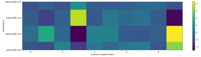
颜色越浅表示权重越高,这里面有sw特征对隐层第4个节点,pl特征对隐层第10个节点的权重较高,可以初步判断这两个特征对于判别一个鸢尾花的品种比较重要。
四、调参
1. 单层隐层
通过调整参数比如hidden_layer_sizes来分析精度随着它的变化的情况。
这里选用一层隐层,节点个数从1变化到100
#调整隐层节点个数
%matplotlib inline
import matplotlib.pyplot as plt
import numpy as np

hidden_lst = []
train_score = []
test_score = []
for hidden in range(1, 101):
    mlp = MLP(solver='lbfgs', random_state=1, hidden_layer_sizes=[hidden],\
     		  max_iter=1000)
    mlp.fit(X_train, y_train)
    hidden_lst.append(hidden)
    train_score.append(mlp.score(X_train, y_train))
    test_score.append(mlp.score(X_test, y_test))

plt.figure(figsize=(20, 5))
plt.plot(hidden_lst, train_score,label="train_score")
plt.plot(hidden_lst, test_score,label="test_score ")
plt.ylabel("Accuracy")
plt.xlabel("hidden_num")
plt.legend()
print("Max accuracy of train set: {0}, min accuracy: {1}, mean accuracy: {2}".format(max(train_score), min(train_score),\
                                                                                     np.mean(train_score)))
print("Max accuracy of test  set: {0}, min accuracy: {1}, mean accuracy: {2}".format(max(test_score), min(test_score),\
                                                                                     np.mean(test_score)))

>>>
Max accuracy of train set: 1.0, min accuracy: 0.36607142857142855, mean accuracy: 0.9594642857142859
Max accuracy of test  set: 1.0, min accuracy: 0.23684210526315788, mean accuracy: 0.9578947368421052
可以发现,训练集和测试集上的最大精度达到100%,最小精度分别为0.37, 0.24,平均精度都在0.95左右。
精度曲线
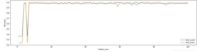
所以,实际上将隐层节点设置在10个左右就可以得到很好的精度,模型也简单。
2. 多层隐层
首先是双层隐层,每个隐层的节点个数为10
mlp = MLP(solver='lbfgs', random_state=1, hidden_layer_sizes=[10,10], max_iter=1000)
mlp.fit(X_train, y_train)

print("Accuracy on training set: {:.3f}".format(mlp.score(X_train, y_train)))
print("Accuracy on testing  set: {:.3f}".format(mlp.score(X_test, y_test)))

>>>
Accuracy on training set: 0.991
Accuracy on testing  set: 1.000
然后我们将第二个隐层的节点数调整为100
mlp = MLP(solver='lbfgs', random_state=1, hidden_layer_sizes=[10,100], max_iter=1000)
mlp.fit(X_train, y_train)

print("Accuracy on training set: {:.3f}".format(mlp.score(X_train, y_train)))
print("Accuracy on testing  set: {:.3f}".format(mlp.score(X_test, y_test)))
>>>
Accuracy on training set: 0.982
Accuracy on testing  set: 1.000
精度有所下降,如果我们再将层数改为三层,每层10个节点的话
mlp = MLP(solver='lbfgs', random_state=1, hidden_layer_sizes=[10,10,10], max_iter=1000)
mlp.fit(X_train, y_train)

print("Accuracy on training set: {:.3f}".format(mlp.score(X_train, y_train)))
print("Accuracy on testing  set: {:.3f}".format(mlp.score(X_test, y_test)))

>>>
Accuracy on training set: 0.795
Accuracy on testing  set: 0.605
发现精度大大下降,层数变多,计算的次数变多,拟合更加困难。
3. 调整隐层个数
我们通过调整隐层个数从1到50,来分析精度的变化
hidden_lst_up = []
train_score_up = []
test_score_up = []
h = [10]
for hidden in range(51):
    mlp = MLP(solver='lbfgs', random_state=1, hidden_layer_sizes=h, max_iter=5000)
    mlp.fit(X_train, y_train)
    hidden_lst_up.append(hidden)
    train_score_up.append(mlp.score(X_train, y_train))
    test_score_up.append(mlp.score(X_test, y_test))
    h.append(10)
plt.figure(figsize=(10, 5))
plt.plot(hidden_lst_up, train_score_up,label="train_score")
plt.plot(hidden_lst_up, test_score_up,label="test_score ")
plt.ylabel("Accuracy")
plt.xlabel("hidden_num")
plt.legend()
print("Max accuracy of train set: {0}, min accuracy: {1}, mean accuracy: {2}".format(max(train_score_up), min(train_score_up),\
                                                                                     np.mean(train_score_up)))
print("Max accuracy of test  set: {0}, min accuracy: {1}, mean accuracy: {2}".format(max(test_score_up), min(test_score_up),\
                                                                                     np.mean(test_score_up)))

>>>
Max accuracy of train set: 0.9910714285714286, min accuracy: 0.30357142857142855, mean accuracy: 0.5087535014005601
Max accuracy of test  set: 1.0, min accuracy: 0.23684210526315788, mean accuracy: 0.43292053663570695

当隐层个数增大是,精度下降的十分明显,但也有意外之处,当隐层个数为26时,精度意外的好。
print(np.array(list(enumerate(train_score_up))))
print(np.array(list(enumerate(test_score_up))))

>>>
[[ 0.          0.98214286]
 [ 1.          0.99107143]
 [ 2.          0.79464286]
 [ 3.          0.97321429]
 [ 4.          0.97321429]
 [ 5.          0.99107143]
 [ 6.          0.96428571]
 [ 7.          0.41071429]
 [ 8.          0.875     ]
 [ 9.          0.33035714]
 [10.          0.30357143]
 [11.          0.875     ]
 [12.          0.63392857]
 [13.          0.33035714]
 [14.          0.5625    ]
 [15.          0.36607143]
 [16.          0.36607143]
 [17.          0.58035714]
 [18.          0.69642857]
 [19.          0.36607143]
 [20.          0.33035714]
 [21.          0.69642857]
 [22.          0.69642857]
 [23.          0.36607143]
 [24.          0.36607143]
 [25.          0.36607143]
 [26.          0.97321429]
 [27.          0.36607143]
 [28.          0.36607143]
 [29.          0.36607143]
 [30.          0.36607143]
 [31.          0.36607143]
 [32.          0.36607143]
 [33.          0.36607143]
 [34.          0.36607143]
 [35.          0.36607143]
 [36.          0.36607143]
 [37.          0.36607143]
 [38.          0.36607143]
 [39.          0.36607143]
 [40.          0.36607143]
 [41.          0.36607143]
 [42.          0.36607143]
 [43.          0.36607143]
 [44.          0.36607143]
 [45.          0.36607143]
 [46.          0.36607143]
 [47.          0.36607143]
 [48.          0.36607143]
 [49.          0.36607143]
 [50.          0.36607143]]
>>>
[[ 0.          1.        ]
 [ 1.          1.        ]
 [ 2.          0.60526316]
 [ 3.          1.        ]
 [ 4.          1.        ]
 [ 5.          1.        ]
 [ 6.          1.        ]
 [ 7.          0.28947368]
 [ 8.          0.78947368]
 [ 9.          0.34210526]
 [10.          0.42105263]
 [11.          1.        ]
 [12.          0.76315789]
 [13.          0.34210526]
 [14.          0.71052632]
 [15.          0.23684211]
 [16.          0.23684211]
 [17.          0.68421053]
 [18.          0.57894737]
 [19.          0.23684211]
 [20.          0.34210526]
 [21.          0.57894737]
 [22.          0.57894737]
 [23.          0.23684211]
 [24.          0.23684211]
 [25.          0.23684211]
 [26.          0.94736842]
 [27.          0.23684211]
 [28.          0.23684211]
 [29.          0.23684211]
 [30.          0.23684211]
 [31.          0.23684211]
 [32.          0.23684211]
 [33.          0.23684211]
 [34.          0.23684211]
 [35.          0.23684211]
 [36.          0.23684211]
 [37.          0.23684211]
 [38.          0.23684211]
 [39.          0.23684211]
 [40.          0.23684211]
 [41.          0.23684211]
 [42.          0.23684211]
 [43.          0.23684211]
 [44.          0.23684211]
 [45.          0.23684211]
 [46.          0.23684211]
 [47.          0.23684211]
 [48.          0.23684211]
 [49.          0.23684211]
 [50.          0.23684211]]
小结
神经网络模型可以达到很高的精度,但这依赖于参数的调整,特别是隐层数目和隐层节点数目;
神经网络的非线性拟合功能很强,虽然是基于梯度下降法来获取系数权重,但是还是有点黑箱功能。