CHAPTER 13 Dependency Parsing

CHAPTER 13 Dependency Parsing

Speech and Language Processing ed3 读书笔记

dependency grammars: the syntactic structure of a sentence is described solely in terms of the words (or lemmas) in a sentence and an associated inventory of directed binary grammatical relations that hold among the words.

Relations among the words are illustrated above the sentence with directed, labeled arcs from heads to dependents. We call this a typed dependency structure because the labels are drawn from a fixed inventory of grammatical relations.

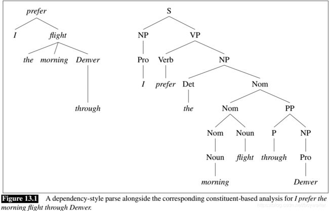
Figure 13.1 shows the same dependency analysis as a tree alongside its corresponding phrase-structure analysis of the kind given in Chapter 10.

One advantage of dependency grammars is that the arguments of a word are directly linked to it.

A major advantage of dependency grammars is their ability to deal with languages that are morphologically rich and have a relatively free word order. A dependency grammar approach abstracts away from word-order information, representing only the information that is necessary for the parse.

An additional practical motivation for a dependency-based approach is that the head-dependent relations provide an approximation to the semantic relationship between predicates and their arguments that makes them directly useful for many applications such as coreference resolution, question answering and information extraction. Constituent-based approaches to parsing provide similar information, but it often has to be distilled from the trees via techniques such as the head finding rules discussed in Chapter 10.

13.1 Dependency Relations

The traditional linguistic notion of grammatical relation provides the basis for the binary relations that comprise these dependency structures. The arguments to these relations consist of a head and a dependent. The head word of a constituent was the central organizing word of a larger constituent (e.g, the primary noun in a noun phrase, or verb in a verb phrase). The remaining words in the constituent are either direct, or indirect, dependents of their head. In dependency-based approaches, the head-dependent relationship is made explicit by directly linking heads to the words that are immediately dependent on them.

In addition to specifying the head-dependent pairs, dependency grammars allow us to further classify the kinds of grammatical relations, or grammatical function, in terms of the role that the dependent plays with respect to its head. Familiar notions such as subject, direct object and indirect object are among the kind of relations we have in mind.

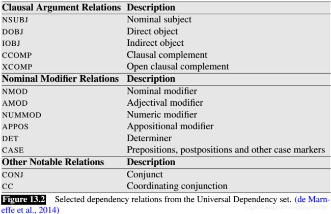
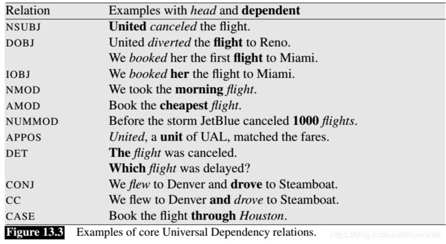
The Universal Dependencies project (Nivre et al., 2016b) provides an inventory of dependency relations that are linguistically motivated, computationally useful, and cross-linguistically applicable. Fig. 13.2 shows a subset of the relations from this effort. Fig. 13.3 provides some example sentences illustrating selected relations.

The core set of frequently used relations can be broken into two sets: clausal relations that describe syntactic roles with respect to a predicate (often a verb), and modifier relations that categorize the ways that words that can modify their heads.

13.2 Dependency Formalisms

A dependency tree is a directed graph that satisfies the following constraints:

1. There is a single designated root node that has no incoming arcs.
2. With the exception of the root node, each vertex has exactly one incoming arc.
3. There is a unique path from the root node to each vertex in $V$ .

13.2.1 Projectivity

An arc from a head to a dependent is said to be projective if there is a path from the head to every word that lies between the head and the dependent in the sentence. A dependency tree is then said to be projective if all the arcs that make it up are projective.

Consider the following example.

A dependency tree is projective if it can be drawn with no crossing edges.

Our concern with projectivity arises from two related issues. First, the most widely used English dependency treebanks were automatically derived from phrase-structure treebanks through the use of head-finding rules (Chapter 10). The trees generated in such a fashion are guaranteed to be projective since they’re generated from context-free grammars.

Second, there are computational limitations to the most widely used families of parsing algorithms. The transition-based approaches discussed in Section 13.4 can only produce projective trees, hence any sentences with non-projective structures will necessarily contain some errors. This limitation is one of the motivations for the more flexible graph-based parsing approach described in Section 13.5.

13.3 Dependency Treebanks

The translation process from constituent to dependency structures has two subtasks: identifying all the head-dependent relations in the structure and identifying the correct dependency relations for these relations. Here’s a simple and effective algorithm from Xia and Palmer (2001).

1. Mark the head child of each node in a phrase structure, using the appropriate head rules.
2. In the dependency structure, make the head of each non-head child depend on the head of the head-child.

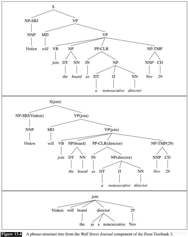
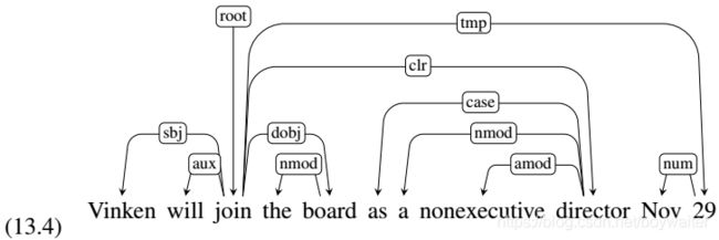
When a phrase-structure parse contains additional information in the form of grammatical relations and function tags, as in the case of the Penn Treebank, these tags can be used to label the edges in the resulting tree. When applied to the parse tree in Fig. 13.4, this algorithm would produce the dependency structure in Fig. 13.4.

13.4 Transition-Based Dependency Parsing

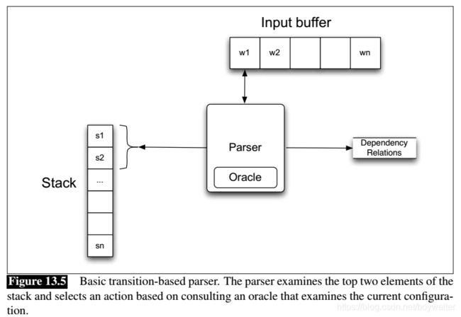
Our first approach to dependency parsing is motivated by a stack-based approach called shift-reduce parsing originally developed for analyzing programming languages (Aho and Ullman, 1972). This classic approach is simple and elegant, employing a context-free grammar, a stack, and a list of tokens to be parsed. Input tokens are successively shifted onto the stack and the top two elements of the stack are matched against the right-hand side of the rules in the grammar; when a match is found the matched elements are replaced on the stack (reduced) by the non-terminal from the left-hand side of the rule being matched. In adapting this approach for dependency parsing, we forgo the explicit use of a grammar and alter the reduce operation so that instead of adding a non-terminal to a parse tree, it introduces a dependency relation between a word and its head. More specifically, the reduce action is replaced with two possible actions: assert a head-dependent relation between the word at the top of the stack and the word below it, or vice versa. Figure 13.5 illustrates the basic operation of such a parser.

A key element in transition-based parsing is the notion of a configuration which consists of a stack, an input buffer of words, or tokens, and a set of relations representing a dependency tree. Given this framework, the parsing process consists of a sequence of transitions through the space of possible configurations. The goal of this process is to find a final configuration where all the words have been accounted for and an appropriate dependency tree has been synthesized.

To implement such a search, we’ll define a set of transition operators, which when applied to a configuration produce new configurations. Given this setup, we can view the operation of a parser as a search through a space of configurations for a sequence of transitions that leads from a start state to a desired goal state. At the start of this process we create an initial configuration in which the stack contains the ROOT node, the word list is initialized with the set of the words or lemmatized tokens in the sentence, and an empty set of relations is created to represent the parse. In the final goal state, the stack and the word list should be empty, and the set of relations will represent the final parse.

In the standard approach to transition-based parsing, the operators used to produce new configurations are surprisingly simple and correspond to the intuitive actions one might take in creating a dependency tree by examining the words in a single pass over the input from left to right (Covington, 2001):

• Assign the current word as the head of some previously seen word,
• Assign some previously seen word as the head of the current word,
• Or postpone doing anything with the current word, adding it to a store for later processing.

To make these actions more precise, we’ll create three transition operators that will operate on the top two elements of the stack:

• LEFTARC: Assert a head-dependent relation between the word at the top of stack and the word directly beneath it; remove the lower word from the stack.
• RIGHTARC: Assert a head-dependent relation between the second word on the stack and the word at the top; remove the word at the top of the stack;
• SHIFT: Remove the word from the front of the input buffer and push it onto the stack.

This particular set of operators implements what is known as the arc standard approach to transition-based parsing (Covington 2001, Nivre 2003). There are two notable characteristics to this approach: the transition operators only assert relations between elements at the top of the stack, and once an element has been assigned its head it is removed from the stack and is not available for further processing. As we’ll see, there are alternative transition systems which demonstrate different parsing behaviors, but the arc standard approach is quite effective and is simple to implement.

To assure that these operators are used properly we’ll need to add some preconditions to their use. First, since, by definition, the ROOT node cannot have any incoming arcs, we’ll add the restriction that the LEFTARC operator cannot be applied when ROOT is the second element of the stack. Second, both reduce operators require two elements to be on the stack to be applied. Given these transition operators and preconditions, the specification of a transition-based parser is quite simple. Fig. 13.6 gives the basic algorithm.

At each step, the parser consults an oracle (we’ll come back to this shortly) that provides the correct transition operator to use given the current configuration. It then applies that operator to the current configuration, producing a new configuration. The process ends when all the words in the sentence have been consumed and the ROOT node is the only element remaining on the stack.

The efficiency of transition-based parsers should be apparent from the algorithm. The complexity is linear in the length of the sentence since it is based on a single left to right pass through the words in the sentence. More specifically, each word must first be shifted onto the stack and then later reduced.

Note that unlike the dynamic programming and search-based approaches discussed in Chapters 12 and 13, this approach is a straightforward greedy algorithm—the oracle provides a single choice at each step and the parser proceeds with that choice, no other options are explored, no backtracking is employed, and a single parse is returned in the end.
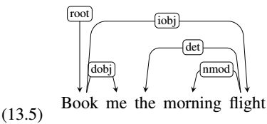
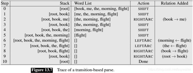
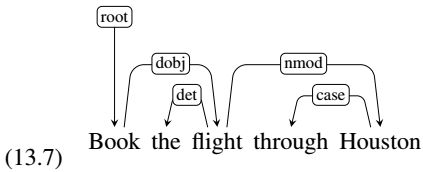
Figure 13.7 illustrates the operation of the parser with the sequence of transitions leading to a parse for the following example.

There are several important things to note when examining sequences such as the one in Figure 13.7. First, the sequence given is not the only one that might lead to a reasonable parse. In general, there may be more than one path that leads to the same result, and due to ambiguity, there may be other transition sequences that lead to different equally valid parses.

Second, we are assuming that the oracle always provides the correct operator at each point in the parse — an assumption that is unlikely to be true in practice. As a result, given the greedy nature of this algorithm, incorrect choices will lead to incorrect parses since the parser has no opportunity to go back and pursue alternative choices. Section 13.4.2 will introduce several techniques that allow transition-based approaches to explore the search space more fully.

Finally, for simplicity, we have illustrated this example without the labels on the dependency relations. To produce labeled trees, we can parameterize the LEFTARC and RIGHTARC operators with dependency labels, as in LEFTARC(NSUBJ) or RIGHTARC(DOBJ). This is equivalent to expanding the set of transition operators from our original set of three to a set that includes LEFTARC and RIGHTARC operators for each relation in the set of dependency relations being used, plus an additional one for the SHIFT operator. This, of course, makes the job of the oracle more difficult since it now has a much larger set of operators from which to choose.

13.4.1 Creating an Oracle

State-of-the-art transition-based systems use supervised machine learning methods to train classifiers that play the role of the oracle. Given appropriate training data, these methods learn a function that maps from configurations to transition operators.

As with all supervised machine learning methods, we will need access to appropriate training data and we will need to extract features useful for characterizing the decisions to be made. The source for this training data will be representative treebanks containing dependency trees. The features will consist of many of the same features we encountered in Chapter 8 for part-of-speech tagging, as well as those used in Chapter 12 for statistical parsing models.

Generating Training Data

Let’s revisit the oracle from the algorithm in Fig. 13.6 to fully understand the learning problem. The oracle takes as input a configuration and returns as output a transition operator. Therefore, to train a classifier, we will need configurations paired with transition operators (i.e., LEFTARC, RIGHTARC, or SHIFT). Unfortunately, treebanks pair entire sentences with their corresponding trees, and therefore they don’t directly provide what we need.

To generate the required training data, we will employ the oracle-based parsing algorithm in a clever way. We will supply our oracle with the training sentences to be parsed along with their corresponding reference parses from the treebank. To produce training instances, we will then simulate the operation of the parser by running the algorithm and relying on a new training oracle to give us correct transition operators for each successive configuration.

To see how this works, let’s first review the operation of our parser. It begins with a default initial configuration where the stack contains the ROOT, the input list is just the list of words, and the set of relations is empty. The LEFTARC and RIGHTARC operators each add relations between the words at the top of the stack to the set of relations being accumulated for a given sentence. Since we have a gold-standard reference parse for each training sentence, we know which dependency relations are valid for a given sentence. Therefore, we can use the reference parse to guide the selection of operators as the parser steps through a sequence of configurations.

To be more precise, given a reference parse and a configuration, the training oracle proceeds as follows:

• Choose LEFTARC if it produces a correct head-dependent relation given the reference parse and the current configuration,
• Otherwise, choose RIGHTARC if (1) it produces a correct head-dependent relation given the reference parse and (2) all of the dependents of the word at the top of the stack have already been assigned,
• Otherwise, choose SHIFT.

The restriction on selecting the RIGHTARC operator is needed to ensure that a word is not popped from the stack, and thus lost to further processing, before all its dependents have been assigned to it.

More formally, during training the oracle has access to the following information:

• A current configuration with a stack $S$ and a set of dependency relations $R_c$
• A reference parse consisting of a set of vertices $V$ and a set of dependency relations $R_p$

Given this information, the oracle chooses transitions as follows:

LEFTARC®: if $(S_{1}r{S}_2)\in R_p$
RIGHTARC®: if $(S_{2}r{S}_1)\in R_p$ and $\forall r^{\prime },ws.t.(S_1{r}^{\prime }w)\in R_p$ then $(S_1{r}^{\prime }w)\in R_c$
SHIFT: otherwise

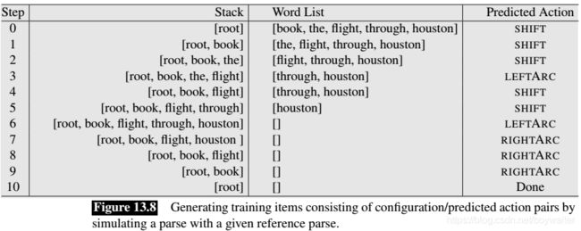
Let’s walk through some steps of this process with the following example as shown in Fig. 13.8.

We derive appropriate training instances consisting of configuration-transition pairs from a treebank by simulating the operation of a parser in the context of a reference dependency tree. We can deterministically record correct parser actions at each step as we progress through each training example, thereby creating the training set we require.

Features

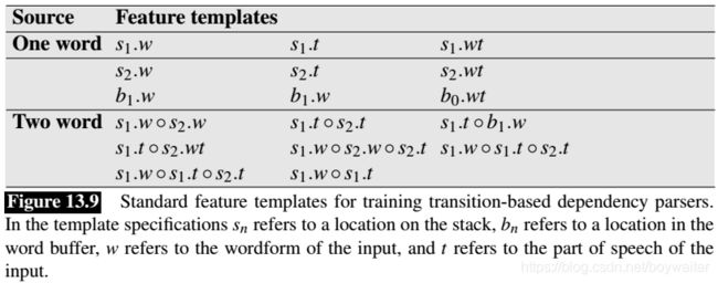
Feature templates allow us to automatically generate large numbers of specific features from a training set. Figure 13.9 gives a baseline set of feature templates that have been employed in various state-of-the-art systems (Zhang and Clark 2008,Huang and Sagae 2010,Zhang and Nivre 2011).

Note that some of these features make use of dynamic features — features such as head words and dependency relations that have been predicted at earlier steps in the parsing process, as opposed to features that are derived from static properties of the input.

Learning
Over the years, the dominant approaches to training transition-based dependency parsers have been multinomial logistic regression and support vector machines, both of which can make effective use of large numbers of sparse features of the kind described in the last section. More recently, neural network, or deep learning, approaches of the kind described in Chapter 8 have been applied successfully to transition-based parsing (Chen and Manning, 2014). These approaches eliminate the need for complex, hand-crafted features and have been particularly effective at overcoming the data sparsity issues normally associated with training transition-based parsers.

13.4.2 Advanced Methods in Transition-Based Parsing

The basic transition-based approach can be elaborated in a number of ways to improve performance by addressing some of the most obvious flaws in the approach.

Alternative Transition Systems

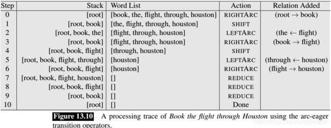
A frequently used alternative is the arc eager transition system. The arc eager approach gets its name from its ability to assert rightward relations much sooner than in the arc standard approach. To see this, let’s revisit the arc standard trace of Example 13.7, repeated here.

The arc-eager system allows words to be attached to their heads as early as possible, before all the subsequent words
dependent on them have been seen. This is accomplished through minor changes to the LEFTARC and RIGHTARC operators and the addition of a new REDUCE operator.

• LEFTARC: Assert a head-dependent relation between the word at the front of the input buffer and the word at the top of the stack; pop the stack.
• RIGHTARC: Assert a head-dependent relation between the word on the top of the stack and the word at front of the input buffer; shift the word at the front of the input buffer to the stack.
• SHIFT: Remove the word from the front of the input buffer and push it onto the stack.
• REDUCE: Pop the stack.

The LEFTARC and RIGHTARC operators are applied to the top of the stack and the front of the input buffer, instead of the top two elements of the stack as in the arc-standard approach. The RIGHTARC operator now moves the dependent to the stack from the buffer rather than removing it, thus making it available to serve as the head of following words. The new REDUCE operator removes the top element from the stack. Together these changes permit a word to be eagerly assigned its head and still allow it to serve as the head for later dependents. The trace shown in Fig. 13.10 illustrates the new decision sequence for this example.

In addition to demonstrating the arc-eager transition system, this example demonstrates the power and flexibility of the overall transition-based approach. We were able to swap in a new transition system without having to make any changes to the underlying parsing algorithm. This flexibility has led to the development of a diverse set of transition systems that address different aspects of syntax and semantics including: assigning part of speech tags (Choi and Palmer, 2011a), allowing the generation of non-projective dependency structures (Nivre, 2009), assigning semantic roles (Choi and Palmer, 2011b), and parsing texts containing multiple languages (Bhat et al., 2017).

Beam Search

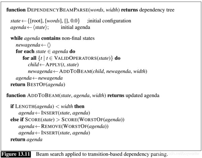
The computational efficiency of the transition-based approach discussed earlier derives from the fact that it makes a single pass through the sentence, greedily making decisions without considering alternatives. Of course, this is also the source of its greatest weakness – once a decision has been made it can not be undone, even in the face of overwhelming evidence arriving later in a sentence. Another approach is to systematically explore alternative decision sequences, selecting the best among those alternatives. The key problem for such a search is to manage the large number of potential sequences. Beam search accomplishes this by combining a breadth-first search strategy with a heuristic filter that prunes the search frontier to stay within a fixed-size beam width.

In applying beam search to transition-based parsing, we’ll elaborate on the algorithm given in Fig. 13.6. Instead of choosing the single best transition operator at each iteration, we’ll apply all applicable operators to each state on an agenda and then score the resulting configurations. We then add each of these new configurations to the frontier, subject to the constraint that there has to be room within the beam. As long as the size of the agenda is within the specified beam width, we can add new configurations to the agenda. Once the agenda reaches the limit, we only add new configurations that are better than the worst configuration on the agenda (removing the worst element so that we stay within the limit). Finally, to insure that we retrieve the best possible state on the agenda, the while loop continues as long as there are non-final states on the agenda.

The beam search approach requires a more elaborate notion of scoring than we used with the greedy algorithm. There, we assumed that a classifier trained using supervised machine learning would serve as an oracle, selecting the best transition operator based on features extracted from the current configuration. Regardless of the specific learning approach, this choice can be viewed as assigning a score to all the possible transitions and picking the best one.
$$\hat{T}(c)=\arg \max Score(t,c)$$
With a beam search we are now searching through the space of decision sequences, so it makes sense to base the score for a configuration on its entire history. More specifically, we can define the score for a new configuration as the score of its predecessor plus the score of the operator used to produce it.
$$\begin{gathered} ConfigScore(c_0)=0.0 \\ ConfigScore(c_i)=ConfigScore(c_{i-1})+Score(t_i,c_{i-1}) \end{gathered}$$
This score is used both in filtering the agenda and in selecting the final answer. The new beam search version of transition-based parsing is given in Fig. 13.11.

13.5 Graph-Based Dependency Parsing

Given a sentence $S$ we’re looking for the best dependency tree in ${\mathcal{G}}_s$, the space of all possible trees for that sentence, that maximizes some score.
$$\hat{T}(S)={\mathrm{argmax}}_{t\in {\mathcal{G}}_S}score(t,S)$$
The overall score for a tree can be viewed as a function of the scores of the parts of the tree. The focus of this section is on edge-factored approaches where the score for a tree is based on the scores of the edges that comprise the tree.
$$score(t,S)=\sum _{e\in t}score(e)$$
There are several motivations for the use of graph-based methods. First, unlike transition-based approaches, these methods are capable of producing non-projective trees. Although projectivity is not a significant issue for English, it is definitely a problem for many of the world’s languages. A second motivation concerns parsing accuracy, particularly with respect to longer dependencies. Empirically, transition-based methods have high accuracy on shorter dependency relations but accuracy declines significantly as the distance between the head and dependent increases (McDonald and Nivre, 2011). Graph-based methods avoid this difficulty by scoring entire trees, rather than relying on greedy local decisions.

The following section examines a widely-studied approach based on the use of a maximum spanning tree (MST) algorithm for weighted, directed graphs. We then discuss features that are typically used to score trees, as well as the methods used to train the scoring models.

13.5.1 Parsing

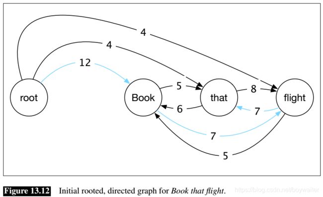
The approach described here uses an efficient greedy algorithm to search for optimal spanning trees in directed graphs. Given an input sentence, it begins by constructing a fully-connected, weighted, directed graph where the vertices are the input words and the directed edges represent all possible head-dependent assignments. An additional ROOT node is included with outgoing edges directed at all of the other vertices. The weights in the graph reflect the score for each possible head-dependent relation as provided by a model generated from training data. Given these weights, a maximum spanning tree of this graph emanating from the ROOT represents the preferred dependency parse for the sentence. A directed graph for the example Book that flight is shown in Fig. 13.12, with the maximum spanning tree corresponding to the desired parse shown in blue. For ease of exposition, we’ll focus here on unlabeled
dependency parsing. Graph-based approaches to labeled parsing are discussed in Section 13.5.3.

Before describing the algorithm it’s useful to consider two intuitions about directed graphs and their spanning trees. The first intuition begins with the fact that every vertex in a spanning tree has exactly one incoming edge. It follows from this that every connected component of a spanning tree will also have one incoming edge. The second intuition is that the absolute values of the edge scores are not critical to determining its maximum spanning tree. Instead, it is the relative weights of the edges entering each vertex that matters. If we were to subtract a constant amount from each edge entering a given vertex it would have no impact on the choice of the maximum spanning tree since every possible spanning tree would decrease by exactly the same amount.

The first step of the algorithm itself is quite straightforward. For each vertex in the graph, an incoming edge (representing a possible head assignment) with the highest score is chosen. If the resulting set of edges produces a spanning tree then we’re done. More formally, given the original fully-connected graph $G=(V,E)$, a subgraph $T=(V,F)$ is a spanning tree if it has no cycles and each vertex (other than the root) has exactly one edge entering it. If the greedy selection process produces such a tree then it is the best possible one.

Unfortunately, this approach doesn’t always lead to a tree since the set of edges selected may contain cycles. Fortunately, in yet another case of multiple discovery, there is a straightforward way to eliminate cycles generated during the greedy selection phase. Chu and Liu (1965) and Edmonds (1967) independently developed an approach that begins with greedy selection and follows with an elegant recursive cleanup phase that eliminates cycles.

The cleanup phase begins by adjusting all the weights in the graph by subtracting the score of the maximum edge entering each vertex from the score of all the edges entering that vertex. This is where the intuitions mentioned earlier come into play. We have scaled the values of the edges so that the weight of the edges in the cycle have no bearing on the weight of any of the possible spanning trees. Subtracting the value of the edge with maximum weight from each edge entering a vertex results in a weight of zero for all of the edges selected during the greedy selection phase, including all of the edges involved in the cycle.

Having adjusted the weights, the algorithm creates a new graph by selecting a cycle and collapsing it into a single new node. Edges that enter or leave the cycle are altered so that they now enter or leave the newly collapsed node. Edges that do not touch the cycle are included and edges within the cycle are dropped.

Now, if we knew the maximum spanning tree of this new graph, we would have what we need to eliminate the cycle. The edge of the maximum spanning tree directed towards the vertex representing the collapsed cycle tells us which edge to delete to eliminate the cycle. How do we find the maximum spanning tree of this new graph? We recursively apply the algorithm to the new graph. This will either result in a spanning tree or a graph with a cycle. The recursions can continue as long as cycles are encountered. When each recursion completes we expand the collapsed vertex, restoring all the vertices and edges from the cycle with the exception of the single edge to be deleted.

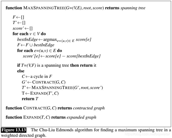
Putting all this together, the maximum spanning tree algorithm consists of greedy edge selection, re-scoring of edge costs and a recursive cleanup phase when needed. The full algorithm is shown in Fig. 13.13.

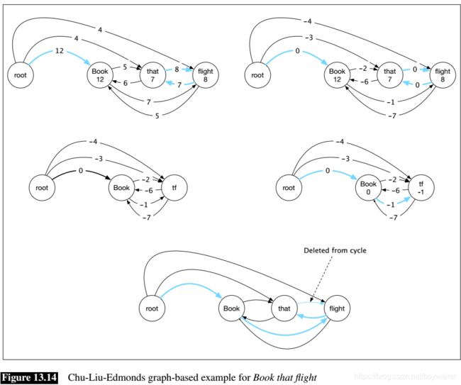
Fig. 13.14 steps through the algorithm with our Book that flight example. The first row of the figure illustrates greedy edge selection with the edges chosen shown in blue (corresponding to the set $F$ in the algorithm). This results in a cycle between that and flight. The scaled weights using the maximum value entering each node are shown in the graph to the right.

Collapsing the cycle between that and flight to a single node (labelled $tf$) and recursing with the newly scaled costs is shown in the second row. The greedy selection step in this recursion yields a spanning tree that links root to book, as well as an edge that links book to the contracted node. Expanding the contracted node, we can see that this edge corresponds to the edge from book to flight in the original graph. This in turn tells us which edge to drop to eliminate the cycle.

On arbitrary directed graphs, this version of the CLE algorithm runs in $O(mn)$ time, where $m$ is the number of edges and $n$ is the number of nodes. Since this particular application of the algorithm begins by constructing a fully connected graph $m=n^2$ yielding a running time of $O(n^3)$. Gabow et al. (1986) present a more efficient implementation with a running time of $O(m+n\log n)$.

13.5.2 Features and Training

Given a sentence, $S$, and a candidate tree, $T$, edge-factored parsing models reduce the score for the tree to a sum of the scores of the edges that comprise the tree.
$$score(S,T)=\sum _{e\in T}score(S,e)$$
Each edge score can, in turn, be reduced to a weighted sum of features extracted from it.
$$score(S,e)=\sum _{i=1}^N{w}_i{f}_i(S,e)$$
Or more succinctly,
$$score(S,e)=w\cdot f$$
Commonly used features include:

• Wordforms, lemmas, and parts of speech of the headword and its dependent.
• Corresponding features derived from the contexts before, after and between the words.
• Word embeddings.
• The dependency relation itself.
• The direction of the relation (to the right or left).
• The distance from the head to the dependent.

As with transition-based approaches, pre-selected combinations of these features are often used as well.

Given a set of features, our next problem is to learn a set of weights corresponding to each. Unlike many of the learning problems discussed in earlier chapters, here we are not training a model to associate training items with class labels, or parser actions. Instead, we seek to train a model that assigns higher scores to correct trees than to incorrect ones. An effective framework for problems like this is to use inference-based learning combined with the perceptron learning rule. In this framework, we parse a sentence (i.e, perform inference) from the training set using some initially random set of initial weights. If the resulting parse matches the corresponding tree in the training data, we do nothing to the weights. Otherwise, we find those features in the incorrect parse that are not present in the reference parse and we lower their weights by a small amount based on the learning rate. We do this incrementally for each sentence in our training data until the weights converge.

More recently, recurrent neural network (RNN) models have demonstrated state-of-the-art performance in shared tasks on multilingual parsing (Zeman et al. 2017, Dozat et al. 2017). These neural approaches rely solely on lexical information in the form of word embeddings, eschewing the use of hand-crafted features such as those described earlier.

13.5.3 Advanced Issues in Graph-Based Parsing

13.6 Evaluation

The most common method for evaluating dependency parsers are labeled and unlabeled attachment accuracy. Labeled attachment refers to the proper assignment of a word to its head along with the correct dependency relation. Unlabeled attachment simply looks at the correctness of the assigned head, ignoring the dependency relation. Given a system output and a corresponding reference parse, accuracy is simply the percentage of words in an input that are assigned the correct head with the correct relation. This metrics are usually referred to as the labeled attachment score (LAS) and unlabeled attachment score (UAS). Finally, we can make use of a label accuracy score (LS), the percentage of tokens with correct labels, ignoring where the relations are coming from.

As an example, consider the reference parse and system parse for the following example shown in Fig. 13.15.

(13.11) Book me the flight through Houston.

The system correctly finds 4 of the 6 dependency relations present in the reference parse and therefore receives an LAS of 2/3. However, one of the 2 incorrect relations found by the system holds between book and flight, which are in a head-dependent relation in the reference parse; therefore the system therefore achieves an UAS of 5/6.

Beyond attachment scores, we may also be interested in how well a system is performing on a particular kind of dependency relation, for example NSUBJ, across a development corpus. Here we can make use of the notions of precision and recall introduced in Chapter 8, measuring the percentage of relations labeled NSUBJ by the system that were correct (precision), and the percentage of the NSUBJ relations present in the development set that were in fact discovered by the system (recall).

We can employ a confusion matrix to keep track of how often each dependency type was confused for another.

13.7 Summary

This chapter has introduced the concept of dependency grammars and dependency parsing. Here’s a summary of the main points that we covered:

• In dependency-based approaches to syntax, the structure of a sentence is described in terms of a set of binary relations that hold between the words in a sentence. Larger notions of constituency are not directly encoded in dependency analyses.
• The relations in a dependency structure capture the head-dependent relationship among the words in a sentence.
• Dependency-based analyses provides information directly useful in further language processing tasks including information extraction, semantic parsing and question answering.
• Transition-based parsing systems employ a greedy stack-based algorithm to create dependency structures.
• Graph-based methods for creating dependency structures are based on the use of maximum spanning tree methods from graph theory.
• Both transition-based and graph-based approaches are developed using supervised machine learning techniques.
• Treebanks provide the data needed to train these systems. Dependency treebanks can be created directly by human annotators or via automatic transformation from phrase-structure treebanks.
• Evaluation of dependency parsers is based on labeled and unlabeled accuracy scores as measured against withheld development and test corpora.