pytorch全连接层梯度链式法则记录
注: 本文仅为查阅网络诸多博客后做出的总结与推理思考,不代表正确观点
雅可比矩阵
向量 X 1 ∗ n X_{1*n} X1∗n通过右乘 W n ∗ m W_{n*m} Wn∗m得到向量 Y 1 ∗ m Y_{1*m} Y1∗m, Y Y Y关于 X X X的偏导数为 W m ∗ n T W^T_{m*n} Wm∗nT。
雅可比矩阵满足链式法则
注意雅可比矩阵满足链式法则只当连续的求导都是在向量之间,引入矩阵之后不满足链式法则
一个例子说明雅可比矩阵的链式法则:
X 1 ∗ n ⋅ ( W n ∗ m 1 ) = Y 1 ∗ m ( 1 ) X_{1*n}\cdot(W^1_{n*m})=Y_{1*m}(1) X1∗n⋅(Wn∗m1)=Y1∗m(1)
Y 1 ∗ m ⋅ ( W 2 m ∗ p ) = Z 1 ∗ p ( 2 ) Y_{1*m}\cdot(W^2{m*p})=Z_{1*p}(2) Y1∗m⋅(W2m∗p)=Z1∗p(2)
链式法则表明下式成立,
d Z / d X = d Z / d Y ∗ d Y / d X dZ/dX=dZ/dY*dY/dX dZ/dX=dZ/dY∗dY/dX
即 d Z / d X = W p ∗ m 2 T ⋅ ( W m ∗ n 1 T ) dZ/dX=W^{2T}_{p*m}\cdot(W^{1T}_{m*n}) dZ/dX=Wp∗m2T⋅(Wm∗n1T)
可以证明上式成立,把(1)代入(2)式得,
X 1 ∗ n ⋅ ( W n ∗ m 1 ) ⋅ ( W m ∗ p 2 ) = Z 1 ∗ p X_{1*n}\cdot(W^1_{n*m})\cdot(W^2_{m*p})=Z_{1*p} X1∗n⋅(Wn∗m1)⋅(Wm∗p2)=Z1∗p
根据雅可比矩阵定义可知 d Z / d X = W p ∗ m 2 T ⋅ ( W m ∗ n 1 T ) dZ/dX=W^{2T}_{p*m}\cdot(W^{1T}_{m*n}) dZ/dX=Wp∗m2T⋅(Wm∗n1T)
pytorch代码验证如下,由于某个向量梯度求出来之后是为了能够乘以一个学习率然后直接和该向量相减进行学习,所以需要梯度的维度和向量维度匹配,最简单的办法就是引入一个1*输出维度的雅可比矩阵然后应用链式法则,也即Pytorch代码中的loss.backward(loss_like的ones Tensor)
# torch grad test
# -------------------------------------------
input_dim = 2
output_dim1 = 3
output_dim2 = 2

x = torch.randn(input_dim, requires_grad=True)
w1 = torch.randn((input_dim, output_dim1), requires_grad=True)
w2 = torch.randn((output_dim1, output_dim2), requires_grad=True)
label = torch.randn(output_dim2)
y1 = x.matmul(w1)
y1.retain_grad()
y2 = y1.matmul(w2)
loss = y2 - label
loss.backward(torch.ones_like(loss))
print('y1.grad: ', y1.grad)
print('our y1.grad: ', np.ones_like(loss.detach().numpy()).dot(w2.detach().numpy().T))
print('x.grad: ', x.grad)
print('our y2.grad: ', np.ones_like(loss.detach().numpy()).dot(w2.detach().numpy().T).dot(w1.detach().numpy().T))

--------------------output------------------------------
y1.grad:  tensor([-2.8673, -0.0941, -1.0313])
our y1.grad:  [-2.8672557  -0.09413806 -1.0312822 ]
x.grad:  tensor([-5.1732,  2.5583])
our y2.grad:  [-5.17317    2.5583477]
对权重求导
有了上述观点以后注意到loss如果对某一层权重求导,先应用雅可比矩阵链式法则对该层输出求导,然后利用该层输出对该层权重求导,这已经不叫链式法则了。
X 1 ∗ n ⋅ ( W n ∗ m 1 ) = Y 1 ∗ m ( 1 ) X_{1*n}\cdot(W^1_{n*m})=Y_{1*m}(1) X1∗n⋅(Wn∗m1)=Y1∗m(1)
根据(1)式求 d Y / d W 1 dY/dW^1 dY/dW1,
因为梯度要和权重维度一致,所以易得 d Y / d W = [ X T , . . . m − 2 个 X T , X T ] n ∗ m dY/dW=[X^T, ...m-2个X^T, X^T]_{n*m} dY/dW=[XT,...m−2个XT,XT]n∗m
当经由反向传播求对于权重的梯度时,比如输出是 Z 1 ∗ p Z_{1*p} Z1∗p,那么 d Z / d Y = M 1 ∗ m dZ/dY=M_{1*m} dZ/dY=M1∗m,这里链式法则乘了一个loss_like的ones矩阵
此时 d Y / d W 1 = [ X T , . . . m − 2 个 X T , X T ] n ∗ m ∗ M n ∗ m dY/dW^1=[X^T, ...m-2个X^T, X^T]_{n*m}*M_{n*m} dY/dW1=[XT,...m−2个XT,XT]n∗m∗Mn∗m
这里 M n ∗ m M_{n*m} Mn∗m代表用 M 1 ∗ m M_{1*m} M1∗m组合出来的一个矩阵,然后直接对应点乘而不是矩阵相乘
pytorch代码验证如下,
# torch grad test
# -------------------------------------------
input_dim = 2
output_dim1 = 3
output_dim2 = 2

x = torch.randn(input_dim, requires_grad=True)
w1 = torch.randn((input_dim, output_dim1), requires_grad=True)
w2 = torch.randn((output_dim1, output_dim2), requires_grad=True)
label = torch.randn(output_dim2)
y1 = x.matmul(w1)
y1.retain_grad()
y2 = y1.matmul(w2)
loss = y2 - label
loss.backward(torch.ones_like(loss))
print('w2.grad: ', w2.grad)
last_jac = np.ones_like(loss.detach().numpy())
last_jacs = last_jac
for i in range(w2.size()[0]-1):
    last_jacs = np.vstack((last_jacs, last_jac))
input_array = y1.detach().numpy().reshape(-1, 1)
input_arrays = input_array
for i in range(w2.size()[1]-1):
    input_arrays = np.hstack((input_arrays, input_array))
print('our w2.grad: ', input_arrays * last_jacs)
print('y1.grad: ', y1.grad)
print('our y1.grad: ', np.ones_like(loss.detach().numpy()).dot(w2.detach().numpy().T))
print('w1.grad: ', w1.grad)
last_jac = y1.grad.numpy()
last_jacs = last_jac
for i in range(w1.size()[0]-1):
    last_jacs = np.vstack((last_jacs, last_jac))
input_array = x.detach().numpy().reshape(-1, 1)
input_arrays = input_array
for i in range(w1.size()[1]-1):
    input_arrays = np.hstack((input_arrays, input_array))
print('our w1.grad: ', input_arrays * last_jacs)
print('x.grad: ', x.grad)
print('our y2.grad: ', np.ones_like(loss.detach().numpy()).dot(w2.detach().numpy().T).dot(w1.detach().numpy().T))

--------------------------output----------------------------
w2.grad:  tensor([[ 0.2581,  0.2581],
        [-0.4644, -0.4644],
        [-1.0143, -1.0143]])
our w2.grad:  [[ 0.2581184   0.2581184 ]
 [-0.46440646 -0.46440646]
 [-1.0143005  -1.0143005 ]]
y1.grad:  tensor([ 0.5938, -0.6923,  1.2869])
our y1.grad:  [ 0.59384376 -0.6922908   1.2869087 ]
w1.grad:  tensor([[-0.3074,  0.3583, -0.6661],
        [ 0.3067, -0.3576,  0.6647]])
our w1.grad:  [[-0.3073509   0.35830334 -0.66605496]
 [ 0.3067317  -0.35758147  0.6647131 ]]
x.grad:  tensor([2.7224, 1.1200])
our y2.grad:  [2.7224424 1.12001  ]
python+numpy实现simple autograd
查阅pytorch源代码以及pytorch tutorial官方提供的autograd示例猜测推理pytorch autograd结构如下
基本原理,pytorch记录前向过程中的每一步操作,然后在反向传播的时候借由链式法则求得对每个参数的导数。
网络的实质只是一堆运算,基本运算包括加法,乘法,sum(降维)和expand(升维)。所以理论上只需要这些运算即可完成网络的前馈与反向传播。但是矩阵运算可以加速,所以基于基本运算封装了很多运算,一方面提高运算速度,一方面增多用户接口方便使用。
根据基本原理知道,首先要有一个记录前向操作的tapes,这个tapes记录每一次操作的inputs,outputs和操作函数,采用一个list结构存放即可,先操作先进。
然后在反向传播的时候loss.backward可以看到pytorch源码调用了c自动微分引擎实现自动微分,根据提供的示例代码猜测每一个pytorch提供的能自动微分的函数里面都有一个类似示例里的propagate函数,这个函数是forward函数里的一个闭包,输入反向传播来的某一层的微分,与该层对每个参数的微分相作用(不同的操作函数实现不同的作用可能是点乘矩阵乘法,参考上两节对向量和权重的求导)。
对记录的tapes反过来,对其中每一条内容,根据对应的propagate求出对应的梯度,对同一变量的梯度采取相加策略(链式法则对同一变量梯度也有这一步y=a+b; c=y*b; dc/db=dy/db * b + db/db * y)。
采取某种结构记录下来每个参数的梯度即可
综上,猜测pytorch的loss.backward()时调用自动微分引擎,反向遍历tapes并基于每个可自动微分函数的类propagate函数实现自动微分,将梯度结果保存到tensor.grad变量中。
当然pytorch的autograd机制比这复杂得多,这只是简化版的理解而已
#!/usr/bin/env python3.6
# -*- coding:utf-8 -*-

import torch
from typing import List, NamedTuple, Callable, Dict, Optional


_name: int = 0
def fresh_name() -> str:
    """ create a new unique name for a variable: v0, v1, v2 """
    global _name
    r = f'v{_name}'
    _name += 1
    return r


class Variable:
    def __init__(self, value: torch.Tensor, name: str = None):
        self.value = value
        self.name = name or fresh_name()
        print(f'{self.name} = {value}')

    # We need to start with some tensors whose values were not computed
    # inside the autograd. This function constructs leaf nodes.
    @staticmethod
    def constant(value: torch.Tensor, name: str = None):
        r = Variable(value, name)
        print(f'{r.name} = {value}')
        return r

    def __repr__(self):
        return repr(self.value)

    # This performs a pointwise multiplication of a Variable, tracking gradients
    def __mul__(self, rhs: 'Variable') -> 'Variable':
        # defined later in the notebook
        return operator_mul(self, rhs)

    def __add__(self, rhs: 'Variable') -> 'Variable':
        return operator_add(self, rhs)

    def sum(self, name: Optional[str] = None) -> 'Variable':
        return operator_sum(self, name)

    def expand(self, sizes: List[int]) -> 'Variable':
        return operator_expand(self, sizes)


class TapeEntry(NamedTuple):
    # names of the inputs to the original computation
    inputs : List[str]
    # names of the outputs of the original computation
    outputs: List[str]
    # apply chain rule
    propagate: 'Callable[[List[Variable]], List[Variable]]'


gradient_tape : List[TapeEntry] = []


def reset_tape():
  gradient_tape.clear()
  global _name
  _name = 0 # reset variable names too to keep them small.


def operator_mul(self: Variable, rhs: Variable) -> Variable:
    if isinstance(rhs, float) and rhs == 1.0:
        # peephole optimization
        return self

    # define forward
    r = Variable(self.value * rhs.value)
    print(f'{r.name} = {self.name} * {rhs.name}')

    # record what the inputs and outputs of the op were
    inputs = [self.name, rhs.name]
    outputs = [r.name]

    # define backprop
    def propagate(dL_doutputs: List[Variable]):
        dL_dr, = dL_doutputs

        dr_dself = rhs  # partial derivative of r = self*rhs
        dr_drhs = self  # partial derivative of r = self*rhs

        # chain rule propagation from outputs to inputs of multiply
        dL_dself = dL_dr * dr_dself
        dL_drhs = dL_dr * dr_drhs
        dL_dinputs = [dL_dself, dL_drhs]
        return dL_dinputs

    # finally, we record the compute we did on the tape
    gradient_tape.append(TapeEntry(inputs=inputs, outputs=outputs, propagate=propagate))
    return r


def operator_add(self : Variable, rhs: Variable) -> Variable:
    # Add follows a similar pattern to Mul, but it doesn't end up
    # capturing any variables.
    r = Variable(self.value + rhs.value)
    print(f'{r.name} = {self.name} + {rhs.name}')
    def propagate(dL_doutputs: List[Variable]):
        dL_dr, = dL_doutputs
        dr_dself = 1.0
        dr_drhs = 1.0
        dL_dself = dL_dr * dr_dself
        dL_drhs = dL_dr * dr_drhs
        return [dL_dself, dL_drhs]
    gradient_tape.append(TapeEntry(inputs=[self.name, rhs.name], outputs=[r.name], propagate=propagate))
    return r


# sum is used to turn our matrices into a single scalar to get a loss.
# expand is the backward of sum, so it is added to make sure our Variable
# is closed under differentiation. Both have rules similar to mul above.
def operator_sum(self: Variable, name: Optional[str]) -> 'Variable':
    r = Variable(torch.sum(self.value), name=name)
    print(f'{r.name} = {self.name}.sum()')
    def propagate(dL_doutputs: List[Variable]):
        dL_dr, = dL_doutputs
        size = self.value.size()
        return [dL_dr.expand(*size)]
    gradient_tape.append(TapeEntry(inputs=[self.name], outputs=[r.name], propagate=propagate))
    return r


def operator_expand(self: Variable, sizes: List[int]) -> 'Variable':
    assert(self.value.dim() == 0) # only works for scalars
    r = Variable(self.value.expand(sizes))
    print(f'{r.name} = {self.name}.expand({sizes})')
    def propagate(dL_doutputs: List[Variable]):
        dL_dr, = dL_doutputs
        return [dL_dr.sum()]
    gradient_tape.append(TapeEntry(inputs=[self.name], outputs=[r.name], propagate=propagate))
    return r


def grad(L, desired_results: List[Variable]) -> List[Variable]:
    # this map holds dL/dX for all values X
    dL_d : Dict[str, Variable] = {}
    # It starts by initializing the 'seed' dL/dL, which is 1
    dL_d[L.name] = Variable(torch.ones(()))
    print(f'd{L.name} ------------------------')

    # look up dL_dentries. If a variable is never used to compute the loss,
    # we consider its gradient None, see the note below about zeros for more information.
    def gather_grad(entries: List[str]):
        # 当某个偏导数为0时,不用继续反向传播浪费计算能力,所以后续在反向传播的时候会先判断上一层偏导是不是全零
        # 但是判断一个很大的矩阵是否全零没有判断是否为None快,所以返回None效率更高
        return [dL_d[entry] if entry in dL_d else None for entry in entries]

    # propagate the gradient information backward
    for entry in reversed(gradient_tape):
        dL_doutputs = gather_grad(entry.outputs)
        if all(dL_doutput is None for dL_doutput in dL_doutputs):
            # 假如有如下
            # c = a * b
            # e = a + f
            # de/db理论上是全零偏导
            # 看一下根据代码的反向传播过程,
            # 第一步,可以得到de/da, de/df
            # 第二步,首先会判断de/dc的值存不存在,第一步过后并没有产生该值所以不存在,
            # 理论上来讲de/dc是全零,反向传播回去de/db也是全零,但是如果已知是全零还反向传播回去属于浪费算力
            # 因此会先判断是否全零,而判断全零比判断None更耗时,所以就不返回全零而是返回None
            # optimize for the case where some gradient pathways are zero. See
            # The note below for more details.
            continue

        # perform chain rule propagation specific to each compute
        dL_dinputs = entry.propagate(dL_doutputs)

        # Accululate the gradient produced for each input.
        # Each use of a variable produces some gradient dL_dinput for that
        # use. The multivariate chain rule tells us it is safe to sum
        # all the contributions together.
        for input, dL_dinput in zip(entry.inputs, dL_dinputs):
            if input not in dL_d:
                dL_d[input] = dL_dinput
            else:
                dL_d[input] += dL_dinput

    # print some information to understand the values of each intermediate
    for name, value in dL_d.items():
        print(f'd{L.name}_d{name} = {value.name}')
    print(f'------------------------')

    return gather_grad(desired.name for desired in desired_results)


a_global, b_global = torch.rand(4), torch.rand(4)

def simple(a, b):
    t = a + b
    return t * b

reset_tape() # reset any compute from other cells
a = Variable.constant(a_global, name='a')
b = Variable.constant(b_global, name='b')
loss = simple(a, b)
da, db = grad(loss, [a, b])
print("da", da)
print("db", db)
给自己的备注,注意里面自己的中文注释
python+numpy实现全连接层
依据上面自动反向传播的简单基本框架,分析知要实现全连接层的反向传播只需再实现一个矩阵乘法的反向传播即可
接下来用自己实现的全连接层真实训练一个非线性函数用来拟合sin函数,分析知道还需要有非线性激活函数和loss函数,基于梯度简单的想法采用relu函数,loss使用mse并实现两者的反向传播自动微分
有了网络反向传播还需要实现优化器,使用最简单的SGD,而且是最简单的一个样本的SGD
实现之后训练网络并与pytorch做对比
网络的初始化权重尤为重要,另外SGD在该问题上的表现并不好,不稳定而且对学习率控制要求高,采用Adam会更好,初始化权重如果不对也训练不出来,采用pytorch全连接层默认参数初始化
pytorch代码
注意为了做对比实验使用了batch_size=1, shuffle=False, SGD优化器
import torch
import numpy as np
import torch.nn as nn
import torch.nn.functional as F
import matplotlib.pyplot as plt
from torch.utils.data import TensorDataset, DataLoader


class Net(nn.Module):
    def __init__(self):
        super(Net, self).__init__()
        self.fc1 = nn.Linear(1, 10)
        self.fc2 = nn.Linear(10, 100)
        self.fc3 = nn.Linear(100, 10)
        self.fc4 = nn.Linear(10, 1)

    def forward(self, x):
        x = self.fc1(x)
        x = F.relu(x)
        x = self.fc2(x)
        x = F.relu(x)
        x = self.fc3(x)
        x = F.relu(x)
        x = self.fc4(x)

        return x


if __name__ == '__main__':
    net = Net()
    optimizer = torch.optim.SGD(net.parameters(), lr=0.01)
    schedule = torch.optim.lr_scheduler.StepLR(optimizer, step_size=500, gamma=0.1)
    losses = []
    x = np.linspace(-10, 10, 500)
    x = x.reshape(-1, 1)
    y = np.sin(x)
    y = y.reshape(-1, 1)
    x = np.asarray(x, np.float32)
    x = torch.from_numpy(x)
    y = np.asarray(y, np.float32)
    label = torch.from_numpy(y)
    dataset = TensorDataset(x, label)
    dataloader = DataLoader(dataset, batch_size=1, shuffle=False)
    for i in range(10):
        for input, output in dataloader:
            pred = net(input)
            loss = F.mse_loss(pred, output)
            losses.append(loss.item())
            optimizer.zero_grad()
            loss.backward()
            optimizer.step()
        schedule.step()
    plt.plot(losses)
    plt.show()
    plt.plot(x.numpy(), y, 'g')
    plt.plot(x.numpy(), net(x).detach().numpy(), 'r')

    plt.show()
结果如下,
自己实现的全连接层,采取pytorch tutorial提供的autograd框架,现在原框架上实现一些要用到的函数和反向传播,再实现全连接层和优化器
simplenaiveautogradimplementation.py
#!/usr/bin/env python3.6
# -*- coding:utf-8 -*-

import torch
import numpy as np
from typing import List, NamedTuple, Callable, Dict, Optional


_name: int = 0
def fresh_name() -> str:
    """ create a new unique name for a variable: v0, v1, v2 """
    global _name
    r = f'v{_name}'
    _name += 1
    return r


class Variable:
    def __init__(self, value: torch.Tensor, name: str = None):
        self.value = value
        self.name = name or fresh_name()
        print(f'{self.name} = {value}')

    # We need to start with some tensors whose values were not computed
    # inside the autograd. This function constructs leaf nodes.
    @staticmethod
    def constant(value: torch.Tensor, name: str = None):
        r = Variable(value, name)
        print(f'{r.name} = {value}')
        return r

    def __repr__(self):
        return repr(self.value)

    # This performs a pointwise multiplication of a Variable, tracking gradients
    def __mul__(self, rhs: 'Variable') -> 'Variable':
        # defined later in the notebook
        return operator_mul(self, rhs)

    def __add__(self, rhs: 'Variable') -> 'Variable':
        return operator_add(self, rhs)

    def sum(self, name: Optional[str] = None) -> 'Variable':
        return operator_sum(self, name)

    def expand(self, sizes: List[int]) -> 'Variable':
        return operator_expand(self, sizes)

    def vectorMatMul(self, weights):
        return operator_vectorMatMul(self, weights)

    def mseLoss(self, label):
        return mseLoss(self, label)


class TapeEntry(NamedTuple):
    # names of the inputs to the original computation
    inputs : List[str]
    # names of the outputs of the original computation
    outputs: List[str]
    # apply chain rule
    propagate: 'Callable[[List[Variable]], List[Variable]]'


gradient_tape : List[TapeEntry] = []


def reset_tape():
    gradient_tape.clear()
    global _name
    _name = 0 # reset variable names too to keep them small.


def operator_mul(self: Variable, rhs: Variable) -> Variable:
    if isinstance(rhs, float) and rhs == 1.0:
        # peephole optimization
        return self

    # define forward
    r = Variable(self.value * rhs.value)
    print(f'{r.name} = {self.name} * {rhs.name}')

    # record what the inputs and outputs of the op were
    inputs = [self.name, rhs.name]
    outputs = [r.name]

    # define backprop
    def propagate(dL_doutputs: List[Variable]):
        dL_dr, = dL_doutputs

        dr_dself = rhs  # partial derivative of r = self*rhs
        dr_drhs = self  # partial derivative of r = self*rhs

        # chain rule propagation from outputs to inputs of multiply
        dL_dself = dL_dr * dr_dself
        dL_drhs = dL_dr * dr_drhs
        dL_dinputs = [dL_dself, dL_drhs]
        return dL_dinputs

    # finally, we record the compute we did on the tape
    gradient_tape.append(TapeEntry(inputs=inputs, outputs=outputs, propagate=propagate))
    return r


def operator_add(self : Variable, rhs: Variable) -> Variable:
    # Add follows a similar pattern to Mul, but it doesn't end up
    # capturing any variables.
    r = Variable(self.value + rhs.value)
    print(f'{r.name} = {self.name} + {rhs.name}')
    def propagate(dL_doutputs: List[Variable]):
        dL_dr, = dL_doutputs
        dr_dself = 1.0
        dr_drhs = 1.0
        dL_dself = dL_dr * dr_dself
        dL_drhs = dL_dr * dr_drhs
        return [dL_dself, dL_drhs]
    gradient_tape.append(TapeEntry(inputs=[self.name, rhs.name], outputs=[r.name], propagate=propagate))
    return r


def operator_vectorMatMul(self, weights):
    assert self.value.ndim == 1
    assert self.value.size()[0] == weights.value.size()[0]
    r = Variable(torch.from_numpy(self.value.numpy().dot(weights.value.numpy())))
    print(f'{r.name} = {self.name}.dot({weights.name})')
    def propagate(dL_doutputs):
        dL_dr, = dL_doutputs
        dL_dself_val = dL_dr.value.numpy().dot(weights.value.numpy().T)
        dL_dself = Variable(torch.from_numpy(dL_dself_val))
        last_jac = dL_dr.value.numpy()
        last_jacs = last_jac
        for i in range(weights.value.size()[0] - 1):
            last_jacs = np.vstack((last_jacs, last_jac))
        input_array = self.value.numpy().reshape(-1, 1)
        input_arrays = input_array
        for i in range(weights.value.size()[1] - 1):
            input_arrays = np.hstack((input_arrays, input_array))
        dL_dweights_val = torch.from_numpy(input_arrays * last_jacs)
        dL_dweights = Variable(dL_dweights_val)
        return [dL_dself, dL_dweights]
    gradient_tape.append(TapeEntry(inputs=[self.name, weights.name], outputs=[r.name], propagate=propagate))
    return r


def mseLoss(self, label):
    r_val = torch.from_numpy(self.value.numpy() - label.value.numpy()) ** 2
    r = Variable(r_val)
    print(f"{r.name} = {self.name}.mseLoss({label.name})")
    def propagate(dL_doutputs):
        dL_dr, = dL_doutputs
        dL_dself_val = dL_dr.value.numpy() * 2 * (self.value.numpy() - label.value.numpy())
        dL_dself = Variable(torch.from_numpy(dL_dself_val))
        dL_dlabel_val = torch.from_numpy(dL_dr.value.numpy() * -2 * (self.value.numpy() - label.value.numpy()))
        dL_dlabel = Variable(dL_dlabel_val)
        return [dL_dself, dL_dlabel]
    gradient_tape.append(TapeEntry(inputs=[self.name, label.name], outputs=[r.name], propagate=propagate))
    return r


def relu(self):
    val = self.value.numpy()
    val[val < 0] = 0
    r_val = torch.from_numpy(val)
    r = Variable(r_val)
    print(f"{r.name} = relu({self.name})")
    def propagate(dL_doutputs):
        dL_dr, = dL_doutputs
        dL_dself_val = torch.from_numpy(dL_dr.value.numpy() * (np.asarray(self.value.numpy() > 0, np.float32)))
        dL_dself = Variable(dL_dself_val)
        return [dL_dself]
    gradient_tape.append(TapeEntry(inputs=[self.name], outputs=[r.name], propagate=propagate))
    return r


# sum is used to turn our matrices into a single scalar to get a loss.
# expand is the backward of sum, so it is added to make sure our Variable
# is closed under differentiation. Both have rules similar to mul above.
def operator_sum(self: Variable, name: Optional[str]) -> 'Variable':
    r = Variable(torch.sum(self.value), name=name)
    print(f'{r.name} = {self.name}.sum()')
    def propagate(dL_doutputs: List[Variable]):
        dL_dr, = dL_doutputs
        size = self.value.size()
        return [dL_dr.expand(*size)]
    gradient_tape.append(TapeEntry(inputs=[self.name], outputs=[r.name], propagate=propagate))
    return r


def operator_expand(self: Variable, sizes: List[int]) -> 'Variable':
    assert(self.value.dim() == 0) # only works for scalars
    r = Variable(self.value.expand(sizes))
    print(f'{r.name} = {self.name}.expand({sizes})')
    def propagate(dL_doutputs: List[Variable]):
        dL_dr, = dL_doutputs
        return [dL_dr.sum()]
    gradient_tape.append(TapeEntry(inputs=[self.name], outputs=[r.name], propagate=propagate))
    return r


def grad(L, desired_results: List[Variable]) -> List[Variable]:
    # this map holds dL/dX for all values X
    dL_d : Dict[str, Variable] = {}
    # It starts by initializing the 'seed' dL/dL, which is 1
    dL_d[L.name] = Variable(torch.ones_like(L.value))
    print(f'd{L.name} ------------------------')

    # look up dL_dentries. If a variable is never used to compute the loss,
    # we consider its gradient None, see the note below about zeros for more information.
    def gather_grad(entries: List[str]):
        # 当某个偏导数为0时,不用继续反向传播浪费计算能力,所以后续在反向传播的时候会先判断上一层偏导是不是全零
        # 但是判断一个很大的矩阵是否全零没有判断是否为None快,所以返回None效率更高
        return [dL_d[entry] if entry in dL_d else None for entry in entries]

    # propagate the gradient information backward
    for entry in reversed(gradient_tape):
        dL_doutputs = gather_grad(entry.outputs)
        if all(dL_doutput is None for dL_doutput in dL_doutputs):
            # 假如有如下
            # c = a * b
            # e = a + f
            # de/db理论上是全零偏导
            # 看一下根据代码的反向传播过程,
            # 第一步,可以得到de/da, de/df
            # 第二步,首先会判断de/dc的值存不存在,第一步过后并没有产生该值所以不存在,
            # 理论上来讲de/dc是全零,反向传播回去de/db也是全零,但是如果已知是全零还反向传播回去属于浪费算力
            # 因此会先判断是否全零,而判断全零比判断None更耗时,所以就不返回全零而是返回None
            # optimize for the case where some gradient pathways are zero. See
            # The note below for more details.
            continue

        # perform chain rule propagation specific to each compute
        dL_dinputs = entry.propagate(dL_doutputs)

        # Accululate the gradient produced for each input.
        # Each use of a variable produces some gradient dL_dinput for that
        # use. The multivariate chain rule tells us it is safe to sum
        # all the contributions together.
        for input, dL_dinput in zip(entry.inputs, dL_dinputs):
            if input not in dL_d:
                dL_d[input] = dL_dinput
            else:
                dL_d[input] += dL_dinput

    # print some information to understand the values of each intermediate
    for name, value in dL_d.items():
        print(f'd{L.name}_d{name} = {value.name}')
    print(f'------------------------')

    return gather_grad(desired.name for desired in desired_results)


if __name__ == '__main__':
    # a_global, b_global = torch.rand(4), torch.rand(4)
    #
    # def simple(a, b):
    #     t = a + b
    #     return t * b
    #
    # reset_tape() # reset any compute from other cells
    # a = Variable.constant(a_global, name='a')
    # b = Variable.constant(b_global, name='b')
    # loss = simple(a, b)
    # da, db = grad(loss, [a, b])
    # print("da", da)
    # print("db", db)

    a_val = torch.rand(4)
    weights_val = torch.rand((4, 5))
    bias_val = torch.rand(5)

    reset_tape()
    a = Variable(a_val)
    weights = Variable(weights_val)
    bias = Variable(bias_val)
    loss = (a.vectorMatMul(weights)) + bias
    da, dweights, dbias = grad(loss, [a, weights, bias])
    print('da: ', da)
    print('dweights: ', dweights)
    print('dbias: ', dbias)
simplenaivefc.py
# /usr/bin/env python3.6
# -*- coding=utf-8 -*-


import sys
sys.path.append('..')
import torch
import numpy as np
from temp.simplenaiveautogradimplementation import gradient_tape, grad, Variable, reset_tape, relu
import matplotlib.pyplot as plt


class FCLayer(object):
    names = []
    def __init__(self, inputDim, outputDim, name):
        if name in FCLayer.names:
            raise Exception('name deprecated!')
        FCLayer.names.append(name)
        super(FCLayer, self).__init__()
        self.weights = Variable(torch.from_numpy(np.asarray(np.random.uniform(-1, 1, (inputDim, outputDim)) / np.sqrt(inputDim), dtype=np.float32)), name=name+"_weights")
        self.bias = Variable(torch.from_numpy(np.asarray(np.random.uniform(-1, 1, outputDim) / np.sqrt(inputDim), dtype=np.float32)), name=name+"_bias")

    def forward(self, x: Variable):
        return x.vectorMatMul(weights=self.weights) + self.bias


class SGDOptimizer(object):
    def __init__(self, params, lr=0.01):
        self._lr = lr
        self._params = params

    def setLr(self, lr):
        self._lr = lr

    def step(self, loss):
        grads = grad(loss, self._params)
        for param, gradient in zip(self._params, grads):
            new_val = param.value.numpy() - self._lr * gradient.value.numpy()
            param.value = torch.from_numpy(new_val)
            # print(f'--{param.name}----{param.name}----{param.name}----{param.name}----{param.name}----{param.name}--')
            # print(param.value)
            # print(f'--{param.name}----{param.name}----{param.name}----{param.name}----{param.name}----{param.name}--')


if __name__ == '__main__':
    fc_layer1 = FCLayer(1, 10, 'fc1')
    fc_layer2 = FCLayer(10, 100, 'fc2')
    fc_layer3 = FCLayer(100, 10, 'fc3')
    fc_layer4 = FCLayer(10, 1, 'fc4')
    optimizer = SGDOptimizer(params=[fc_layer1.weights, fc_layer1.bias, fc_layer2.weights, fc_layer2.bias,
                                     fc_layer3.weights, fc_layer3.bias, fc_layer4.weights, fc_layer4.bias])
    losses = []
    sample_num = 500
    x = np.linspace(-10, 10, sample_num)
    x = x.reshape(-1, 1)
    y = np.sin(x)
    y = y.reshape(-1, 1)
    x = np.asarray(x, np.float32)
    y = np.asarray(y, np.float32)
    for i in range(10):
        for i in range(sample_num):
            reset_tape()
            cur_sample = x[i]
            cur_label = y[i]
            cur_sample = Variable(torch.from_numpy(cur_sample))
            cur_label = Variable(torch.from_numpy(cur_label))
            pred_y = fc_layer4.forward(relu(fc_layer3.forward(relu(fc_layer2.forward(relu(fc_layer1.forward(cur_sample)))))))
            loss = pred_y.mseLoss(cur_label)
            losses.append(loss.value)
            optimizer.step(loss)
    plt.plot(losses)
    plt.show()
    x = np.linspace(-10, 10, sample_num)
    x = x.reshape(-1, 1)
    y = np.sin(x)
    y = y.reshape(-1, 1)
    x = np.asarray(x, np.float32)
    y = np.asarray(y, np.float32)
    plt.plot(x, y, 'g')
    # plt.show()
    pred_y = []
    for i in range(sample_num):
        cur_sample = Variable(torch.from_numpy(x[i]))
        pred_y.append(fc_layer4.forward(relu(
            fc_layer3.forward(relu(
                fc_layer2.forward(relu(
                    fc_layer1.forward(cur_sample)
                )
                )
            )
            )
        )
        ).value)
    plt.plot(x, pred_y, 'r')
    plt.show()
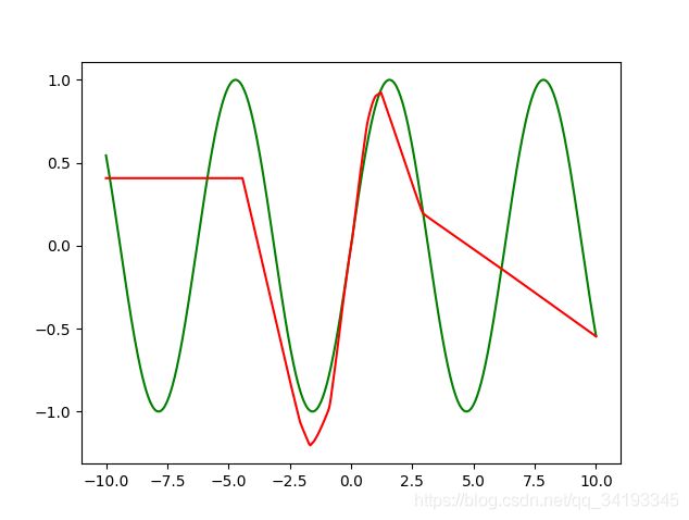
结果如下,

可以看到与pytorch版本的效果几乎一样,证明反向传播过程无误,当然结果并不可重复,因为SGD每一次都会收敛到不同的结果,这里是收敛的比较好的一次
more naive fclayer using numpy+python
上面的autograd是用了一个字典记录grad值的,但是想尝试下能不能直接像pytorch的Tensor一样拿一个grad属性来存梯度值