skimage的基本用法
#skimage
import skimage
import matplotlib.pyplot as plt
import numpy as np
#随机生成500*500的多维数组
random_image = np.random.random([500,500])
plt.imshow(random_image,cmap='gray')
plt.colorbar()

from skimage import data
#加载skimage中的coin数据
coins = data.coins()

print(type(coins),coins.dtype,coins.shape)
plt.imshow(coins,cmap='gray')
plt.colorbar()

#图片基本信息
cat = data.chelsea()
print("图片形状:",cat.shape)
print("最大值,最小值:",cat.min(),cat.max())
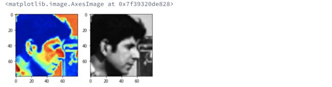
plt.imshow(cat)
plt.colorbar()

#红色通道
plt.imshow(cat[:,:,0])
plt.colorbar()

#在图片上叠加一个红色的方块
cat[10:110,10:110,:] = [255,0,0] #[red,green,blue]
plt.imshow(cat)

#数据类型和像素值
#生成0-1间的2500个数据
linear0 = np.linspace(0,1,2500).reshape((50,50))
#生成0-255之间的2500个数据
linear1 = np.linspace(0,255,2500).reshape(50,50).astype(np.uint8)

print("linear0:",linear0.dtype,linear0.min(),linear0.max())
print("linear1:",linear1.dtype,linear1.min(),linear1.max())

fig,(ax0,ax1) = plt.subplots(1,2)
ax0.imshow(linear0,cmap="gray")
ax1.imshow(linear1,cmap="gray")

#显示图像
image = data.camera()
fig,(ax_jet,ax_gray) = plt.subplots(ncols=2,figsize=(10,5))
#使用不同的color map
ax_jet.imshow(image,cmap='jet')
ax_gray.imshow(image,cmap='gray')

#通过数组切片操作获取人脸区域
face = image[80:160,200:280]
fig,(ax_jet,ax_gray) = plt.subplots(ncols=2)
ax_jet.imshow(face,cmap="jet")
ax_gray.imshow(face,cmap="gray")
#图像的IO操作
from skimage import io
image = io.imread('./images.png')
print(type(image))
plt.imshow(image)
#同时加载多个图像
ic = io.imread_collection('./*.png')
print(type(ic),'\n\n',ic))

f,axes = plt.subplots(nrows=1,ncols=len(ic),figsize(15,10))
#enumerate返回的是带索引的(枚举) 对象
for i,image in enumerate(ic):
    axes[i].imshow(image)
    axes[i].axis('off')

#保存图像
saved_img = ic[0]
io.imsave('./',saved_img)

#色彩转换
#RGB转GRAY
skimage.color.rgb2gray()
#颜色直方图
#直方图是一种快速的描述图像整体像素分布的统计信息
skimage.exposure.histogram
#可以根据直方图选定阈值用于调节图像对比度
直方图是在展平图像上计算的:对于彩色图像,应在每个通道上单独使用该功能,以获得每个颜色通道的直方图。
exposure.histogram()
输入:
图像:数组 输入图像。
nbins:int 用于计算直方图的区间数。整数数组将忽略此值。
返回值:
hist:数组 直方图的值。
bin_centers:数组 bins中心的值。
如果您想在曲线下方填充颜色,请使用fill_between()
#彩色图像直方图
cat = data.chelsea()

#R通道
hist_r,bin_centers_r = exposure.histogram(cat[:,:,0])
#G通道
hist_g,bin_centers_g = exposure.histogram(cat[:,:,1])
#B通道
hist_b,bin_centers_b = exposure.histogram(cat[:,:,2])

fig,(ax_r,ax_g,ax_b) = plt.subplots(ncols=3,figsize=(10,5))
#ax = plt.gca()
ax_r.fill_between(bin_centers_r,hist_r)
ax_g.fill_between(bin_centers_g,hist_g)
ax_b.fill_between(bin_centers_b,hist_b)

对比度
- 增强图像数据的对比度有利于特征的提取,不论是从肉眼还是算法来看都有帮助
- 更改对比范围
skimage.exposure.rescale_intensity(image,in_range=(min,max))
元图数据中,小于min的像素值设为0,大于max的像素值设为255 - 直方图均衡化
自动调整图像的对比度skimage.exposure.equalize_hist(image)
[注意】均衡化后的图像数据范围是[0,1]
#原图像
image = data.camera()
hist,bin_centers = exposure.histogram(image)

#改变对比度
#image中小于10的像素值设为0,大于180的像素值设为255
high_contrast = exposure.rescale_intensity(image,in_range=(10,180))
hist2,bin_center2 = exposure.histogram(high_contrast)
#图像对比
fig,(ax_1,ax_2) = plt.subplots(ncols=2,figsize=(10,5))
ax_1.imshow(image,cmap='gray')
ax_2.imshow(high_contrast,cmap='gray')

fig,(ax_hist1,ax_hist2) = plt.subplots(ncols=2,figsize=(10,5))
ax_hist1.fill_between(bin_centers,hist)
ax_hist2.fill_between(bin_center2,hist2)
skimage.exposure.rescale_intensity(image,in_range = None,out_range = None)
拉伸或收缩其强度水平后返回图像。均匀地重新调整图像强度,使得由in_range给出的最小值和最大值匹配由out_range给出的值。
参数:
image:数组 图像数组。
in_range:2元组(浮点数,浮点数)
最小和最大允许输入图像的强度值。如果为None,则 允许的最小值/最大值设置为输入图像中的实际最小值/最大值。
out_range:2元组(浮点数,浮点数)
输出图像的最小和最大强度值。如果为None,则使用图像数据类型的最小/最大强度。
返回值:
out:数组
重新调整其强度后的图像数组。该图像与输入图像的dtype相同。

直方图均衡化
#直方图均衡化
equalized = exposure.equalize_hist(image)
hist3,bin_center3 = exposure.histogram(equalized)

#图像对比
fig,(ax_1,ax_2) = plt.subplots(ncols=2,figsize=(10,5))
ax_1.imshow(image,cmap='gray')
ax_2.imshow(equalized,cmap='gray')
fig,(ax_hist1,ax_hist2) = plt.subplots(ncols=2,figsize=(10,5))
ax_hist1.fill_between(bin_centers,hist)
ax_hist2.fill_between(bin_center3,hist3)
在这里exposure.equalize_hist(image)效果更好,衣服上的褶皱能很清楚的看到。
滤波分析
图像滤波
- 滤波是处理图像数据的常用基础操作
- 滤波操作可以去除图像中的噪声点,由此增强图像的特征。
中值滤波
skimage.filters.rank.median()
如图:把像素点排序,取中位数,用中位数填充。是一种平滑处理。

#中值滤波
from skimage.morphology import disk
from skimage.filters.rank import median

img = data.camera()
med1 = median(img,disk(3)) #3*3的中值滤波
med2 = median(img,disk(20)) #5*5的中值滤波

#图像对比
fig,(ax_1,ax_2,ax_3) = plt.subplots(ncols=3,figsize=(15,10))
ax_1.imshow(img,cmap='gray')
ax_2.imshow(med1,cmap='gray')
ax_3.imshow(med2,cmap='gray')

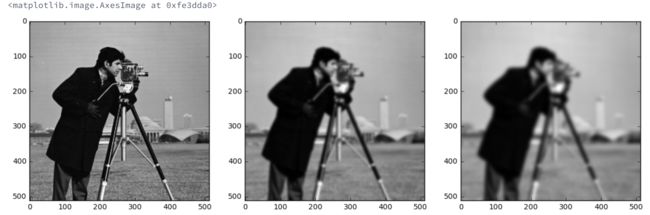
高斯滤波
skimage.filters.gaussian
from skimage import data
from skimage.morphology import disk
from skimage.filters import gaussian

img = data.camera()
gas1 = gaussian(img, sigma=3) # sigma=3
gas2 = gaussian(img, sigma=5) # sigma=5

# 图像对比
fig, (ax_1, ax_2, ax_3) = plt.subplots(ncols=3, figsize=(15, 10))
ax_1.imshow(img, cmap='gray')
ax_2.imshow(gas1, cmap='gray')
ax_3.imshow(gas2, cmap='gray')
OpenCV部分
opencv io
img = cv2.imread('./images/messi.jpg', cv2.IMREAD_GRAYSCALE)
cv2.imshow('messi', img)
k = cv2.waitKey(0)
if k == 27:
    # ESC键->关闭窗口
    cv2.destroyAllWindows()
elif k == ord('s'):
    # 's'键->保存灰度图像并关闭窗口
    cv2.imwrite('./output/messi_gray.png', img)
    cv2.destroyAllWindows()
中值滤波
img = cv2.imread('./')
denoise_img1 = cv2.medianBlur(img, ksize=3)
denoise_img2 = cv2.medianBlur(img, ksize=5)

cv2.imshow('original', img)
cv2.imshow('denoised1', denoise_img1)
cv2.imshow('denoised2', denoise_img2)
k = cv2.waitKey(0)
平滑均值滤波
img = cv2.imread('./')
blured_img1 = cv2.blur(img, ksize=(3, 3))
blured_img2 = cv2.blur(img, ksize=(5, 5))

cv2.imshow('original', img)
cv2.imshow('blured1', blured_img1)
cv2.imshow('blured2', blured_img2)
k = cv2.waitKey(0)
平滑高斯滤波
img = data.camera()
gaussian_img1 = cv2.blur(img, ksize=(3, 3))
gaussian_img2 = cv2.blur(img, ksize=(5, 5))

cv2.imshow('original', img)
cv2.imshow('gaussian1', gaussian_img1)
cv2.imshow('gaussian2', gaussian_img2)
k = cv2.waitKey(0)
常用的图像特征
- 颜色特征
from skimage import data, img_as_float, exposure

# 如果需要使用参数nbins,需要将图像数据从[0, 255]转换到[0, 1]
camera = img_as_float(data.camera())

# 颜色直方图
hist, bin_centers = exposure.histogram(camera, nbins=10)
print(hist)
print(bin_centers)

结果如下:
[51199  8554  6922  8834 31923 45742 82660 23862  1470   978]
[ 0.05  0.15  0.25  0.35  0.45  0.55  0.65  0.75  0.85  0.95]
- SIFT 特征 (DAISY特征)
图像形状特征
• 形状特征的表达必须以对图像中物体或区域的分割为基础
• SIFT (Scale-invariant feature transform),在尺度空间中所提取的图像局部
特征点。SIFT特征点提取较为方便,提取速度较快,对于图像的缩放等变换比
较鲁棒,因此得到了广泛的应用。
• http://docs.opencv.org/trunk/da/df5/tutorial_py_sift_intro.html

from skimage.feature import daisy
import matplotlib.pyplot as plt
%matplotlib inline

daisy_feat, daisy_img = daisy(camera,step=180, radius=58, rings=2, histograms=6, visualize=True)
#daisy_feat, daisy_img = daisy(camera, visualize=True)
print(daisy_feat.shape)
plt.imshow(daisy_img)

from skimage.feature import hog
import matplotlib.pyplot as plt
%matplotlib inline

hog_feat, hog_img = hog(camera, visualise=True)
print(hog_feat.shape)
plt.imshow(hog_img)
- skimage -- HOG 特征
图像形状特征
• HOG (Histogram of Oriented Gradient),用于检测物体的特征描述,通过 计算和统计图像局部区域的梯度方向直方图来构建特征
• 由于HOG是在图像的局部方格单元上操作,所以它对图像几何的和光学的形变 都能保持很好的不变性
• 在粗的空域抽样、精细的方向抽样以及较强的局部光学归一化等条件下,只要 行人大体上能够保持直立的姿势,可以容许行人有一些细微的肢体动作,这些 细微的动作可以被忽略而不影响检测效果
• HOG特征特别适合于做图像中的人体检测 http://mccormickml.com/2013/05/09/hog-person-detector-tutorial/
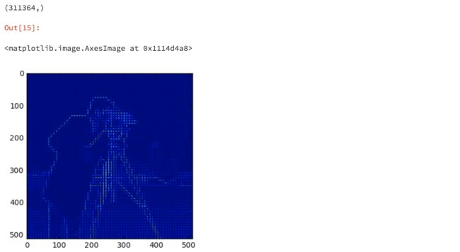
import cv2
image = cv2.imread('./images/messi.jpg',0)
hog = cv2.HOGDescriptor()
hog_feat = hog.compute(image)
print(hog_feat)
print(hog_feat.shape)

结果如下:
[[ 0.1394383 ]
 [ 0.03070632]
 [ 0.02309218]
 ...,
 [ 0.11105878]
 [ 0.15578346]
 [ 0.13455178]]
(3704400, 1)
参考:
• 深度 | 微软亚洲研究院常务副院长郭百宁:计算机视觉的最新研究与应用 http://chuansong.me/n/401296742796
• scikit-image官网 http://scikit-image.org/
• 中值滤波 http://homepages.inf.ed.ac.uk/rbf/HIPR2/median.htm
• 高斯滤波 http://homepages.inf.ed.ac.uk/rbf/HIPR2/gsmooth.htm
• OpenCV 3.2.0 官方教程 http://docs.opencv.org/3.2.0/d6/d00/tutorial_py_root.html