Neural Networks and Deep Learning
This is my notebook when I learn deep learning from Neural Networks and Deep Learning
CHAPTER 1: Using neural nets to recognize handwritten digits
Two important types of artificial neuron (the perceptron and the sigmoid neuron), and the standard learning algorithm for neural networks, known as stochastic gradient descent.
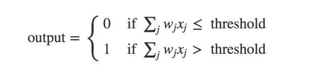
Perceptrons
A perceptron takes several binary inputs, x1,x2,..., and produces a single binary output
-
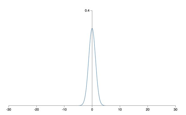
 data distribution
 A small change in the weights or bias of any single perceptron in the network can sometimes cause the output of that perceptron to completely flip. That makes it difficult to see how to gradually modify the weights and biases so that the network gets closer to the desired behaviour.
Sigmoid neuron
Similar to perceptrons, but modified so that small changes in their weights and bias cause only a small change in their output.
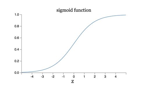
Sigmoid function,σ(w⋅x+b),so output is between 0~1
Sigmoid is a smoothed out perceptron.
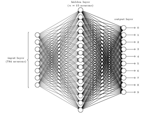
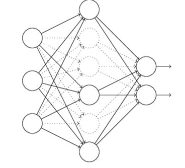
The architecture of neural networks
input layer, hidden layer, output layer
output from one layer is used as input to the next layer. Such networks are called feedforward neural networks
A simple network to classify handwritten digits
A three-layer neural network:
Learning with gradient descent
Denote the corresponding desired output by y=y(x), where y is a 10-dimensional vector. For example, if a particular training image, xx, depicts a 66, then y(x)=(0,0,0,0,0,0,1,0,0,0)T
cost funtion: C(w,b)≡1/2*n∑||y(x)−a||^2
w denotes the collection of all weights in the network, b all the biases, n is the total number of training inputs, a is the vector of outputs from the network when x is input
- SGD: computing ∇Cx for a small sample of randomly chosen training inputs
CHAPTER 2: How the backpropagation algorithm works
As matrix:
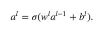
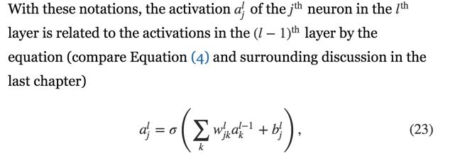
It illustrates how the activations in one layer relate to activations in the previous layer.
For backpropagation to work we need to make two main assumptions:
- The cost function can be written as an average over cost functions Cx for individual training examples, x.
- The cost function can be written as a function of the outputs from the neural network.
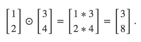
The Hadamard product, s⊙t
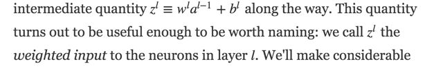
Defenition of Z
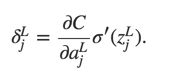
The four fundamental equations behind backpropagation

- An equation for the error in the output layer
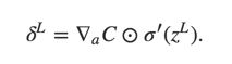 matrix-based
 - An equation for the error in terms of the error in the next layer

By combining these two equations, we can compute the error for any layer in the network. - An equation for the rate of change of the cost with respect to any bias in the network
 bias
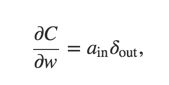
bias - An equation for the rate of change of the cost with respect to any weight in the network
 weight
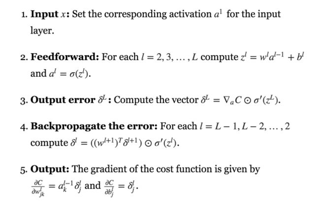
The backpropagation algorithm
Code
__author__ = 'Michael Nielsen '
# http://neuralnetworksanddeeplearning.com/chap1.html

import numpy as np
import random

def sigmoid(z):
    return 1.0/(1.0+np.exp(-z))

def sigmoid_prime(z):
    """Derivative of the sigmoid function."""
    return sigmoid(z)*(1-sigmoid(z))

class Network(object):

    def __init__(self, sizes):
        self.num_layers = len(sizes)
        self.sizes = sizes
        self.biases = [np.random.randn(y, 1) for y in sizes[1:]]
        self.weights = [np.random.randn(y, x)
                        for x, y in zip(sizes[:-1], sizes[1:])]

    def feedforward(self, a):
        """Return the output of the network if "a" is input."""
        for b, w in zip(self.biases, self.weights):
            a = sigmoid(np.dot(w, a)+b)
        return a

    def SGD(self, training_data, epochs, mini_batch_size, eta,
            test_data=None):
        """Train the neural network using mini-batch stochastic
        gradient descent.  The "training_data" is a list of tuples
        "(x, y)" representing the training inputs and the desired
        outputs.  The other non-optional parameters are
        self-explanatory.  If "test_data" is provided then the
        network will be evaluated against the test data after each
        epoch, and partial progress printed out.  This is useful for
        tracking progress, but slows things down substantially."""
        if test_data: n_test = len(test_data)
        n = len(training_data)
        for j in range(epochs):
            random.shuffle(training_data)
            mini_batches = [training_data[k:k+mini_batch_size] for k in range(0, n, mini_batch_size)]
            for mini_batch in mini_batches:
                self.update_mini_batch(mini_batch, eta)
            if test_data:
                print ("Epoch {0}: {1} / {2}".format(j, self.evaluate(test_data), n_test))
            else:
                print ("Epoch {0} complete".format(j))

    def update_mini_batch(self, mini_batch, eta):
        """Update the network's weights and biases by applying
        gradient descent using backpropagation to a single mini batch.
        The "mini_batch" is a list of tuples "(x, y)", and "eta"
        is the learning rate."""
        nabla_b = [np.zeros(b.shape) for b in self.biases]
        nabla_w = [np.zeros(w.shape) for w in self.weights]
        for x, y in mini_batch:
            delta_nabla_b, delta_nabla_w = self.backprop(x, y)
            nabla_b = [nb+dnb for nb, dnb in zip(nabla_b, delta_nabla_b)]
            nabla_w = [nw+dnw for nw, dnw in zip(nabla_w, delta_nabla_w)]
        self.weights = [w-(eta/len(mini_batch))*nw
                        for w, nw in zip(self.weights, nabla_w)]
        self.biases = [b-(eta/len(mini_batch))*nb
                       for b, nb in zip(self.biases, nabla_b)]

    def backprop(self, x, y):
        """Return a tuple ``(nabla_b, nabla_w)`` representing the
        gradient for the cost function C_x.  ``nabla_b`` and
        ``nabla_w`` are layer-by-layer lists of numpy arrays, similar
        to ``self.biases`` and ``self.weights``."""
        nabla_b = [np.zeros(b.shape) for b in self.biases]
        nabla_w = [np.zeros(w.shape) for w in self.weights]
        # feedforward
        activation = x
        activations = [x] # list to store all the activations, layer by layer
        zs = [] # list to store all the z vectors, layer by layer
        for b, w in zip(self.biases, self.weights):
            z = np.dot(w, activation)+b
            zs.append(z)
            activation = sigmoid(z)
            activations.append(activation)
        # backward pass
        delta = self.cost_derivative(activations[-1], y) * \
            sigmoid_prime(zs[-1]) #the first error
        nabla_b[-1] = delta
        nabla_w[-1] = np.dot(delta, activations[-2].transpose())
        # Note that the variable l in the loop below is used a little
        # differently to the notation in Chapter 2 of the book.  Here,
        # l = 1 means the last layer of neurons, l = 2 is the
        # second-last layer, and so on.  It's a renumbering of the
        # scheme in the book, used here to take advantage of the fact
        # that Python can use negative indices in lists.
        for l in range(2, self.num_layers):
            z = zs[-l]
            sp = sigmoid_prime(z)
            delta = np.dot(self.weights[-l+1].transpose(), delta) * sp
            nabla_b[-l] = delta
            nabla_w[-l] = np.dot(delta, activations[-l-1].transpose())
        return (nabla_b, nabla_w)

    def evaluate(self, test_data):
        """Return the number of test inputs for which the neural
        network outputs the correct result. Note that the neural
        network's output is assumed to be the index of whichever
        neuron in the final layer has the highest activation."""
        test_results = [(np.argmax(self.feedforward(x)), y)
                        for (x, y) in test_data]
        return sum(int(x == y) for (x, y) in test_results)

    def cost_derivative(self, output_activations, y):
        """Return the vector of partial derivatives \partial C_x /
        \partial a for the output activations."""
        return (output_activations-y)
The implementation of stochastic gradient descent loops over training examples in a mini-batch. It's possible to modify the backpropagation algorithm so that it computes the gradients for all training examples in a mini-batch simultaneously by matrix.
CHAPTER 3: Improving the way neural networks learn
The cross-entropy cost function
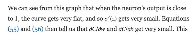
Learning Slowdown
Using quadratic cost as cost function will lead to learning slowdown.
Cross-entropy Cost
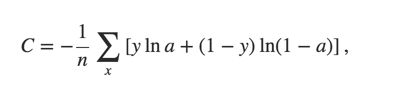
- First, it's non-negative
-
Tends toward zero as the neuron gets better at computing the desired output
Based on this cost function,
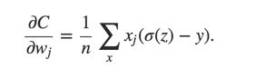 gradient
It's controlled by (a-y),which means if the error gets bigger, the faster the neuron will learn. Thus it avoids the learning slowdown.
Regularization
L2 regularization

Dropout
When we dropout different sets of neurons, it's rather like we're training different neural networks. And so the dropout procedure is like averaging the effects of a very large number of different networks. The different networks will overfit in different ways, and so, hopefully, the net effect of dropout will be to reduce overfitting.
Weight initialization

Will not lead to learning down!
Handwriting recognition revisited: the code
network2.py
Other models of artificial neuron
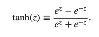
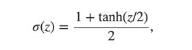
That is tanh is just a rescaled version of the sigmoid function.
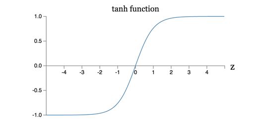
One difference between tanh neurons and sigmoid neurons is that the output from tanh neurons ranges from -1 to 1, not 0 to 1.
CHAPTER 4
A visual proof that neural nets can compute any function