一、概念
Logistic Regression(逻辑回归)是机器学习中一个非常非常常见的模型,在实际生产环境中也常常被使用,是一种经典的分类模型(不是回归模型)。本文主要介绍了Logistic Regression(逻辑回归)模型的原理以及参数估计、公式推导方法。
1、模型构建
在介绍Logistic Regression之前我们先简单说一下线性回归,线性回归的主要思想就是通过历史数据拟合出一条直线,用这条直线对新的数据进行预测
我们知道,线性回归的公式如下:
而对于Logistic Regression来说,其思想也是基于线性回归(Logistic Regression属于广义线性回归模型)。其公式如下:

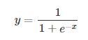
被称作sigmoid函数,我们可以看到,Logistic Regression算法是将线性函数的结果映射到了sigmoid函数中。
sigmoid的函数图形如下:

我们可以看到,sigmoid的函数输出是介于(0,1)之间的,中间值是0.5,于是之前的公式 hθ(x) 的含义就很好理解了,因为 hθ(x) 输出是介于(0,1)之间,也就表明了数据属于某一类别的概率,例如 :
hθ(x)<0.5 则说明当前数据属于A类;
hθ(x)>0.5 则说明当前数据属于B类。
所以我们可以将sigmoid函数看成样本数据的概率密度函数。
有了上面的公式,我们接下来需要做的就是怎样去估计参数 θ 了。

2、极大似然估计
根据上式,接下来我们可以使用概率论中极大似然估计的方法去求解损失函数,首先得到概率函数为:
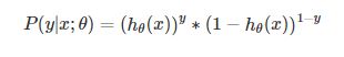
因为样本数据(m个)独立,所以它们的联合分布可以表示为各边际分布的乘积,取似然函数为:

取对数似然函数:

最大似然估计就是要求得使 l(θ) 取最大值时的 θ ,这里可以使用梯度上升法求解。
二、例子
#梯度上升求最大值,梯度下降求最小值
import numpy   as np
import matplotlib.pyplot as plt
import pandas  as pd
import ggplot  as gp

path=u'D:\\PythonStudy\\Ch05\\'
#加载数据集
def loadDataSet():
    dataMat=[];labelMat=[]
    fr=open(path+'testSet.txt')
    for line in fr.readlines():
        lineArr=line.strip().split()
        dataMat.append([1.0,float(lineArr[0]),float(lineArr[1])])
        labelMat.append(int(lineArr[2]))
    return  dataMat,labelMat

def sigmoid(inx):
    return 1.0/(1+np.exp(-inx))
#梯度上升
def gradAscent(dataMatin,classLabels):
    dataMatrix=np.mat(dataMatin)
    labelMat=np.mat(classLabels).T
    m,n=np.shape(dataMatin)
    print("m的值是:{0}".format(m))
    print("n的值是:{0}".format(n))
    alpha=0.0001
    maxCycles=5000
    weights=np.ones((n,1))
    for k in range(maxCycles):
        h=sigmoid(dataMatrix*weights)
        error=(labelMat-h)
        weights=weights+alpha*dataMatrix.T*error
    return  weights

#利用matplotlib.pyplot 画出决策边界画出数据集和logistics回归的最佳拟合直线的函数
def plotWeight(wei):
    weights=wei.getA()   #getA()函数把矩阵变为array的格式
    dataMat,labelMat=loadDataSet()
    dataArr=np.array(dataMat)
    n=np.shape(dataArr)[0]
    xcord1=[];ycordl=[]
    xcord2=[];ycord2=[]
    for  i in range(n):
        if int(labelMat[i])==1:
            xcord1.append(dataArr[i,1]);ycordl.append(dataArr[i,2])
        else:
            xcord2.append(dataArr[i,1]);ycord2.append(dataArr[i,2])
    fig=plt.figure()
    ax=fig.add_subplot(111)
    ax.scatter(xcord1,ycordl,s=30,c='red',marker='s')
    ax.scatter(xcord2,ycord2,s=30,c='green')
    x=np.arange(-3,3,0.1)
    y=(-weights[0]-weights[1]*x)/weights[2]
    ax.plot(x,y)
    plt.xlabel('x1')
    plt.ylabel('x2')
    plt.show()

#注意随机梯度于梯度上升算法的区别
#随机梯度上升算法
#一次仅用一个样本点来更新回归系数,称为随机梯度上升的算法,一次处理 所有的数据
#随机梯度上升算法实现过程
def stocGradAscent0(dataMatrix,classlabels):
    dataMatrix=np.array(dataMatrix)
    m,n=np.shape(dataMatrix)
    alpha=0.01
    weights=np.ones(n)
    for  i in range(m):
        h=sigmoid(sum(dataMatrix[i]*weights))
        error=classlabels[i]-h
        weights=weights+alpha*error*dataMatrix[i]
    weights=np.mat(weights)
    return weights.T

#改进的随机梯度上升
def stocGradAscent1(dataMatrix,classlabels,numIter=150):
    dataMatrix=np.array(dataMatrix)
    m,n=np.shape(dataMatrix)
    weights_x0=[];weights_x1=[];weights_x2=[];weights_ij=[]
    weights=np.ones(n)
    for j in range(numIter):
        dataIndex=list(range(m))
        for  i in range(m):
            alpha=4/(1.0+j+i)+0.01
            randIndex=int(np.random.uniform(0,len(dataIndex)))   #随机生成一个0到len(dataIndex)一个数,用于随度梯度下降
            h=sigmoid(sum(dataMatrix[randIndex]*weights))
            error=classlabels[randIndex]-h
            weights=weights+alpha*error*dataMatrix[randIndex]
            del(dataIndex[randIndex])
            weights_x0.append(weights[0])
            weights_x1.append(weights[1])
            weights_x2.append(weights[2])

    weights_ij.extend(range(1,numIter*m+1))
    weights_dataframe=pd.DataFrame({'weights_x0':weights_x0,'weights_x1':weights_x1,'weights_x2':weights_x2,'weights_ij':weights_ij})

    weights=np.mat(weights)
    return weights.T,weights_dataframe

#matplot描述参数变化情况
def plotDataFrame(weights_dataframe):
    plt.figure()
    plt.plot(weights_dataframe.weights_ij,weights_dataframe.weights_x1,label='weights_x1')
    plt.plot(weights_dataframe.weights_ij,weights_dataframe.weights_x0,label='weights_x0')
    plt.plot(weights_dataframe.weights_ij,weights_dataframe.weights_x2,label='weights_x2')
    plt.legend(loc='upper right')
    plt.xlabel(u"迭代次数", fontproperties='SimHei')
    plt.ylabel(u"参数变化", fontproperties='SimHei')
    plt.title(u"迭代次数显示", fontproperties='SimHei')
    plt.show()

#从疝气病预测病马的死亡率
def classifyVector(Inx,weights):
    prob=sigmoid(sum(Inx*weights))
    if  prob>0.5:
        return 1.0
    else:
        return 0.0
def colicTest():
    frTrain=open(path+'horseColicTraining.txt')
    frTest=open(path+'horseColicTest.txt')
    trainingSet=[];trainLabels=[]
    for  line  in frTrain.readlines():
        currLine=line.strip().split('\t')
        lineArr=[]
        for  i  in range(21):
            lineArr.append(float(currLine[i]))
        trainingSet.append(lineArr)
        trainLabels.append(float(currLine[21]))
    trainWeights,weights_dataframe=stocGradAscent1(np.array(trainingSet), trainLabels,500)
    errorCount=0;numTestVec=0.0
    for line  in frTest.readlines():
        numTestVec+=1.0
        currLine=line.strip().split('\t')
        lineArr=[]
        for i in range(21):
            lineArr.append(float(currLine[i]))
        if int(classifyVector(np.array(lineArr), trainWeights))!=int(currLine[21]):
            errorCount+=1
        errorRate=(float(errorCount))/numTestVec
        print ("the  error rate of this test is :%f"%errorRate)
    return errorRate
def multiTest():
    numTest=10; errorSum=0.0
    for k in range(numTest):
        errorSum+=colicTest()
    print ("after %d iterations the average error rate is :%f"%(numTest,errorSum/float(numTest)))


if  __name__=='__main__':
    dataArr,labelMat=loadDataSet()
    weights=gradAscent(dataArr, labelMat)
    print("梯度生生的参数为:{0}".format(weights))
    plotWeight(weights)

    weights=stocGradAscent0(dataArr, labelMat)
    print("随机梯度生生的参数为:{0}".format(weights))
    plotWeight(weights)

    weights,weights_dataframe=stocGradAscent1(dataArr, labelMat)
    print("改进的随机梯度生生的参数为:{0}".format(weights))
    plotWeight(weights)
    plotDataFrame(weights_dataframe)

    #ggplot描述参数变化情况
    #print(gp.ggplot(weights_dataframe,gp.aes(x='weights_ij',y='weights_x1'))+gp.geom_point(gp.aes(color='red'))+gp.geom_line())
    #print(gp.ggplot(weights_dataframe,gp.aes(x='weights_ij',y='weights_x0'))+gp.geom_point(gp.aes(color='red'))+gp.geom_line())
    #print(gp.ggplot(weights_dataframe,gp.aes(x='weights_ij',y='weights_x2'))+gp.geom_point(gp.aes(color='red'))+gp.geom_line())

    multiTest()
以上案例中所用到的数据集:
testSet.txt------------------------------测试梯度上升法数据集
horseColicTraining.txt--------------疝气病预测的训练数据集
horseColicTest.txt-------------------疝气病预测的测试数据集
结果:
m的值是:100
n的值是:3
梯度生生的参数为:[[ 4.12128936]
 [ 0.47982794]
 [-0.61648878]]
随机梯度生生的参数为:[[ 1.01702007]
 [ 0.85914348]
 [-0.36579921]]
改进的随机梯度生生的参数为:[[14.05218171]
 [ 1.02094074]
 [-2.08521133]]
......
the  error rate of this test is :0.385965
the  error rate of this test is :0.379310
the  error rate of this test is :0.389831
the  error rate of this test is :0.400000
the  error rate of this test is :0.393443
the  error rate of this test is :0.387097
the  error rate of this test is :0.380952
the  error rate of this test is :0.375000
the  error rate of this test is :0.369231
the  error rate of this test is :0.378788
the  error rate of this test is :0.388060
after 10 iterations the average error rate is :0.361194---(预测误差率在30%左右)

梯度上升算法

随机梯度于梯度上升算法

改进的随机梯度上升
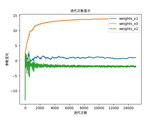
描述参数变化情况