一、差异分析内容及意义
a)随机森林模型(Random Forest)
一种非线性分类器,挖掘变量之间复杂的非线性的相互依赖关系。
意义:找到能够区分两组样品间差异的关键OTU。
b)交叉验证(Cross validation)
对随机森林筛选出的关键OTU组成进行遍历。
意义:以期用最少的OTU数目组合构建一个错误率最低的高效分类器。
c)ROC曲线(接收者操作特征曲线)
属于二元分类算法,用来处理只有两种分类的问题,可以用于选择最佳的判别模型,选择最佳的诊断界限值。
d)LEfSe分析
区别两个或两个以上生物条件;
识别不同丰度的特征以及相关联的类别;
主要计算方式:通过非参数因子KW和秩检验找到丰度差异类群;LDA(线性判别分析)评估每个组分丰度对差异效果的影响大小。
e)Wilcoxon秩和检验分析[又称曼-惠特尼U检验(Mann–Whitney U test)]
两组独立样本非参数检验的一种方法。
可以对两组样品的物种进行显著性差异分析。
f)两组样本Welch’s t-test分析
适用于两组不同方差的样本。
获得在两组中有显著性差异的物种。
g)ANOSIM相似性分析
非参数检验,基于距离(Bray-Curtis等)计算组间差异是否大于组内。
h)Adonis多因素方差分析(置换多因素/非参数多因素方差分析)
半度量(如Bray-Curtis)或度量距离矩阵(如Euclidean)对总方差进行分解,分析不同分组因素对样品差异的解释度,并使用置换检验对划分的统计学意义进行显著性分析。
i)基于差异分析的可视化图表
①多样性指数盒状图(基于非阐述Manny- Whitney计算显著差异)
②基于距离的箱式图(基于multiple Student’s two-sample t-tests判断样本组间差异的显著性)
易于识别异常值、特征值等。
二、差异分析在论文中的描述
a)随机森林模型&ROC曲线
方法描述示例:
Random Forest (RF) analysis was used to find the most discriminatory OTUs between XX with active disease versus XX. As it is unlikely that an OTU present in a minority of samples will have group-related importance, OTUs were only included in the statistical analysis if they were detected in at least 20% of the samples in one of the groups. Prior to actual RF analyses, the microbiome data were transformed via an inverse hyperbolic sine transformation and then mean centered per individual patient. The first step accounts for skewness and can deal with sparse microbiome data. The mean centering per individual diminishes the influence of inter-individual variation.
In the current study, two different RF models were built. The first RF model based on XX different randomly selected subsets, aimed to find the most discriminatory OTUs between XX and XX. The second RF model was performed to demonstrate the contribution of the most discriminatory OTUs in differentiating XX and XX and to test the classification performance of the model in the validation set. The second RF model was based on XX randomly selected subsets. For both RF models, each subset contained all samples from the same individual either in the training set, consisting of 80% of all samples, or in the validation set (the remaining 20%). Thereby, the RF classification model was never trained on part of the measurements of one subject and tested on the remaining measurements of that subject.
The final classification of each sample was determined by a majority of votes (>50%) from XX RF classification models. The final performance of the RF classification model is demonstrated by the receiver operating characteristic (ROC) curve.

结果描述:
We subsequently performed RF analysis to examine whether we could discriminate samples collected during XX and XX based upon the microbiota composition. First, we reduced the data by including only those OTUs (n= XXX) that were present in at least 20% of the XX and/ or XX samples. Subsequently, a first RF analysis was used for the selection of the most discriminatory OTUs between XX and XX samples. The RF-analysis assigned a variable importance score to each OTU, indicating to what extend the OTUs contributed to the model. Based on the variable importance profile, XX OTUs with the highest variable importance scores were selected. The performance of the RF classification model based on the most discriminatory OTUs resulted in an area under the ROC curve (AUC) of 0.82 for the validation set, corresponding to a sensitivity of 0.79 and a specificity of 0.73. The positive predictive value (PPV) and negative predictive value (NPV) were both 0.76.
b)随机森林模型、交叉验证、ROC曲线、Wilcoxn检验:
①方法描述:
We mapped reads from the discovery phase, validation phase and independent diagnosis phase against these represented sequences to generate the discovery OTU frequency profile, validation OTU frequency profile and independent diagnosis frequency profile, respectively. Wilcoxon test was used to determine the significance (p<0.05), based on which XX OTU biomarkers were selected for further analysis. Five-fold cross-validation was performed on a random forest model with default parameters using the XX-OTU abundance profile of training cohort, including XX and XX with liver cirrhosis (assigned as non-HCC cohort) and XX with HCC. Using five trials of the five fold cross-validation, we then obtained the cross-validation error curve. The point with the minimum cross-validation error was viewed as the cut-off point, and the cut-off value was determined via the minimum error plus the SD at the corresponding point. We listed all sets (≤XX) of OTU markers with the error less than the cut-off value and chose the set with the smallest number of OTUs as the optimal set.
POD index was defined as the ratio between the number of randomly generated decision trees that predicted sample as ‘HCC’ and that of healthy controls. The identified optimal set of OTUs was finally used for the calculation of POD index for both the training and testing cohort. And the receiver operating characteristic (ROC) curve was obtained for the evaluation of the constructed models, and the area under the ROC curve (AUC) was used to designate the ROC effect. The detailed script of microbial marker identification and POD construction can be found in the online supplementary methods.
结果的描述:
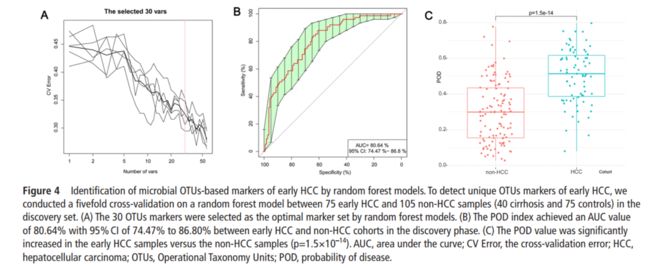
To illustrate the diagnostic value of faecal microbiome for early HCC, we constructed a random forest classifier model that could specifically identify early HCC samples from non-HCC samples. To detect unique OTUs markers of early HCC, we conducted a fivefold cross-validation on a random forest model between XX and XX samples in the discovery phase. The result indicated that the 30 OTU markers were selected as the optimal marker set . The relative abundance of the 30 OTUs markers in each sample from the discovery phase were presented. The corresponding bacterial genera of the 30 OTUs markers are listed in the online. The POD index was calculated using the identified optimal 30 OTUs set for both the discovery cohort and the validation cohort. In the discovery phase, the POD index achieved an AUC value of 80.64% with 95% CI of 74.47% to 86.8% between early HCC and non-HCC cohorts. The POD value was significantly increased in the early HCC samples versus the non-HCC samples (p=1.5×10⁻¹⁴). These data suggested that the POD based on microbial OTUs markers achieved a powerful diagnostic potential for early HCC cohort from the non-HCC cohort.
C)LEfSe

图表描述:
Different structures of adenoma tissue and control tissue microbiota. (A) Taxnomic representation of statistically and biologically consistent diffrernces between Adenoma Tissue and Control Tissue. Differences are represented by the color of the most abundant class (Red indicating Adenoma Tissue, yellow non-significant and green Control Tissue). The diameter of each cicle’s diameter is proportional to the taxon’s abundance. (B) Histogram of the LDA scores for differentially abundant genera.
结果描述:
According to LEfSe analysis, the greatest differences in taxa between the two communities were displayed. ……were have more influence in XX group. ……
温馨提示:
一些差异分析,可以直接在文章中进行描述不用可视化图表体现;
有必要体现在可视化图表中时,需要根据结果在图中进行标注;
在差异分析结果中,分析方法多,结果文件多,因此要根据文章成文情况和撰写内容,依据实际情况进行结果分析及提取。
一些差异分析及模型并非一次即可分析成型,需要基于已有结果,逐步调整分析方案,方能获得理想结果。