BIOS14: ONE-WAY ANOVA(单因素方差分析) using R
NOTES
1 Intruduction of ANOVA
1.1 terminology
If we have 4 groupps of samples, with mean μ 1 , μ 2 , μ 3 , μ 4 \mu_1, \mu_2, \mu_3, \mu_4 μ1,μ2,μ3,μ4, respectively. If we use t-test to test whether the means of 4 population are equle, we have to repeat 6 times t-test.
If all tests are made at some specified significance level (the possibility of error I α \alpha α), the overall level of 6 tests together will be 1 − ( 1 − α ) 6 = 0.625 > > 0.05 1-(1-\alpha)^6 = 0.625 >> 0.05 1−(1−α)6=0.625>>0.05.
Generally speaking, with the increase of the times of carrying on the significant test, the significant level will decrease.
ANOVA (analysis of variance) is used to test equality of multiple overall mean value.
Suppose we want to compare the quality of different industries according to the number of complaints received.
Here, the object be tested (diferent industries) is defined as factor, and the proformence of the factor(the number of complaints received) is defined as treatment. One-way anova means there are only one factor.
1.2 Principles and basic ideas
- describe with plot
Using scatter plot to explore the data, and check the diference. - error separation
SST: Reflecting the error of all datas.
SSE: Reflecting the with-in group error.
SSA: Reflecting the group error. - error analysis
Analyse where the error comes from, with-in group or between group.
1.3 Assumption
- The populations are normal distributions.
- The populations have the same variance.
- observation is independent.
Typically:
H 0 : μ 1 = μ 2 = . . . = μ k H 1 : μ i ≠ μ j f o r s o m e p a i r ( i , j ) H_0: \mu_1=\mu_2=...=\mu_k \\ H_1: \mu_i \ne \mu_j\quad for\ some\ pair(i, j) H0:μ1=μ2=...=μkH1:μi=μjfor some pair(i,j)
Exrcise
Start by installing (if needed) and loading:
- car
- lmtest
- multcomp
One-way anova analysis is used when we want to see if the mean of a continuous variable differs between groups (i.e. between levels of a single categorical variable, a.k.a. factor). It is a generalisation of the t-test, and can be applied to more than two groups. The significance of the categorical variable depends on the relationship between the within-group variance and the among-group variance. If the differences between groups are large compared to the variation within each group, then the categorical variable is likely to be significant. If you are comparing more than two groups, some follow-up analysis (a posthoc test or planned comparison/contrast) is usually necessary to determine exactly which groups differ from each other.
One-way anova with posthoc test
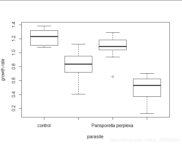
We will start off with an example, an analysis of how Daphnia growth rates depend on what type of parasite individuals are infected with. There were 4 treatments; control and three different species of parasite.
1 Data import and exploration
daphnia = read.csv("daphniagrowth.csv")
boxplot(growth.rate~parasite, data = daphnia)
2 Construct one-way anova model
Believe it or not, but a one-way anova is just another type of linear model. R knows that this data should be analysed using a one-way anova because parasiteis a factor. Because of the flexibility of the linear model using lm(), you need to always be sure that the structure of your dataset is correct before running any analyses! Specifically, if you have any categorical variables with numeric data names (e.g. inbred line ID number or something similar) you must be sure to change them into factors using factor() before building your linear model, otherwise R will treat the analysis as a regression, rather than an anova.
fit.daph = lm(growth.rate~parasite, data=daphnia)
3 Assumptions of one-way anova
- Independent observations
- Normality of the residuals
- Homogeneity of variances
#Independent measurements
> dwtest(fit.daph)

	Durbin-Watson test

data:  fit.daph
DW = 2.0542, p-value = 0.376
alternative hypothesis: true autocorrelation is greater than 0
#Homogeneity of variances and normality of residuals
> par(mfrow=c(2,2))
> plot(fit.daph)
> par(mfrow=c(1,1))
> shapiro.test(fit.daph$residuals)

	Shapiro-Wilk normality test

data:  fit.daph$residuals
W = 0.94661, p-value = 0.05801

> x = fit.daph$residuals
> y = pnorm(summary(x), mean =mean(x, na.rm=TRUE), sd =sd(x, na.rm=TRUE))
> ks.test(x, y)

	Two-sample Kolmogorov-Smirnov test

data:  x and y
D = 0.80833, p-value = 0.0004087
alternative hypothesis: two-sided

> leveneTest(fit.daph)
Levene's Test for Homogeneity of Variance (center = median)
      Df F value Pr(>F)
group  3  0.7041 0.5559
      36
 When plotting the model object, you’ll notice that although the QQ-plot looks pretty much the same as it usually does, the other plots do not. Specifically, the data seems to be distributed along the x-axis in clumps. This is because our predictor variable is now categorical, rather than continuous. Apart from this, the plots should be interpreted in the same was as before (no evidence of outliers in the leverage plot, the red fit line should be more or less flat in the residuals-fitted and scale-location plots).
4 Get results of one-way anova
> anova(fit.daph)
Analysis of Variance Table

Response: growth.rate
          Df Sum Sq Mean Sq F value    Pr(>F)
parasite   3 3.1379 1.04597  32.325 2.571e-10 ***
Residuals 36 1.1649 0.03236
---
Signif. codes:
0 ‘***’ 0.001 ‘**’ 0.01 ‘*’ 0.05 ‘.’ 0.1 ‘ ’ 1
> summary(fit.daph)

Call:
lm(formula = growth.rate ~ parasite, data = daphnia)

Residuals:
     Min       1Q   Median       3Q      Max
-0.41930 -0.09696  0.01408  0.12267  0.31790

Coefficients:
                                  Estimate
(Intercept)                        1.21391
parasiteMetschnikowia bicuspidata -0.41275
parasitePansporella perplexa      -0.13755
parasitePasteuria ramosa          -0.73171
                                  Std. Error
(Intercept)                          0.05688
parasiteMetschnikowia bicuspidata    0.08045
parasitePansporella perplexa         0.08045
parasitePasteuria ramosa             0.08045
                                  t value
(Intercept)                        21.340
parasiteMetschnikowia bicuspidata  -5.131
parasitePansporella perplexa       -1.710
parasitePasteuria ramosa           -9.096
                                  Pr(>|t|)
(Intercept)                        < 2e-16 ***
parasiteMetschnikowia bicuspidata 1.01e-05 ***
parasitePansporella perplexa        0.0959 .
parasitePasteuria ramosa          7.34e-11 ***
---
Signif. codes:
0 ‘***’ 0.001 ‘**’ 0.01 ‘*’ 0.05 ‘.’ 0.1 ‘ ’ 1

Residual standard error: 0.1799 on 36 degrees of freedom
Multiple R-squared:  0.7293,	Adjusted R-squared:  0.7067
F-statistic: 32.33 on 3 and 36 DF,  p-value: 2.571e-10
There is a significant effect of parasites on growth rate. Infected individuals grow less well than the controls.
In the anova() output, keep an eye on the degrees of freedom for your categorical predictor. It should be one less than the number of groups. If you have three or more groups, but the degrees of freedom are listed as equal to1, then your predictor variable is probably coded numerically and you forgot to make it a factor.
The summary() output needs to be interpreted a bit differently for a one-way anova compared to a regression.The levels of a factor are always ordered alphanumerically by default, and the first level gets set as a sort of reference value. That means that the (Intercept) row actually shows the estimated mean for the control treatment in the analysis. The p-value for this row shows whether the control mean value is significantly different from zero or not. In the next row (parasite Metschnikowia bicuspidata), the estimate shows the difference between the mean of this group and the control (intercept value), and whether this specific contrast is significant or not. The third row shows the estimated difference in mean and significance value for a comparison between the P. perplexa group and the control, and so on.
5 Carry out posthoc test
#Posthoc test
> ph.daph = glht(fit.daph, linfct =mcp(parasite="Tukey"))
> summary(ph.daph)

	 Simultaneous Tests for General Linear Hypotheses

Multiple Comparisons of Means: Tukey Contrasts


Fit: lm(formula = growth.rate ~ parasite, data = daphnia)

Linear Hypotheses:
                                                      Estimate
Metschnikowia bicuspidata - control == 0              -0.41275
Pansporella perplexa - control == 0                   -0.13755
Pasteuria ramosa - control == 0                       -0.73171
Pansporella perplexa - Metschnikowia bicuspidata == 0  0.27520
Pasteuria ramosa - Metschnikowia bicuspidata == 0     -0.31895
Pasteuria ramosa - Pansporella perplexa == 0          -0.59415
                                                      Std. Error
Metschnikowia bicuspidata - control == 0                 0.08045
Pansporella perplexa - control == 0                      0.08045
Pasteuria ramosa - control == 0                          0.08045
Pansporella perplexa - Metschnikowia bicuspidata == 0    0.08045
Pasteuria ramosa - Metschnikowia bicuspidata == 0        0.08045
Pasteuria ramosa - Pansporella perplexa == 0             0.08045
                                                      t value
Metschnikowia bicuspidata - control == 0               -5.131
Pansporella perplexa - control == 0                    -1.710
Pasteuria ramosa - control == 0                        -9.096
Pansporella perplexa - Metschnikowia bicuspidata == 0   3.421
Pasteuria ramosa - Metschnikowia bicuspidata == 0      -3.965
Pasteuria ramosa - Pansporella perplexa == 0           -7.386
                                                      Pr(>|t|)
Metschnikowia bicuspidata - control == 0               < 0.001
Pansporella perplexa - control == 0                    0.33354
Pasteuria ramosa - control == 0                        < 0.001
Pansporella perplexa - Metschnikowia bicuspidata == 0  0.00826
Pasteuria ramosa - Metschnikowia bicuspidata == 0      0.00168
Pasteuria ramosa - Pansporella perplexa == 0           < 0.001

Metschnikowia bicuspidata - control == 0              ***
Pansporella perplexa - control == 0
Pasteuria ramosa - control == 0                       ***
Pansporella perplexa - Metschnikowia bicuspidata == 0 **
Pasteuria ramosa - Metschnikowia bicuspidata == 0     **
Pasteuria ramosa - Pansporella perplexa == 0          ***
---
Signif. codes:
0 ‘***’ 0.001 ‘**’ 0.01 ‘*’ 0.05 ‘.’ 0.1 ‘ ’ 1
(Adjusted p values reported -- single-step method)
> cld(ph.daph)
                  control
                      "c"
Metschnikowia bicuspidata
                      "b"
     Pansporella perplexa
                      "c"
         Pasteuria ramosa
                      "a"
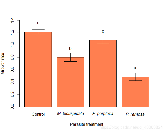
You can also get a summary of the homogenous subsets in your data using cld(ph.daph), same letters means the diference is not significantlly.
6 Illustrate results
> mean.gr = aggregate(list(GR=daphnia$growth.rate), by=list(treat=daphnia$parasite),mean, na.rm=TRUE)
> SE = function(x) sd(x, na.rm=TRUE)/(sqrt(sum(!is.na(x))))
> se.gr = aggregate(list(SE=daphnia$growth.rate), by=list(treat=daphnia$parasite), FUN=SE)
> gr.dat = cbind(mean.gr, SE=se.gr$SE, cld=c("c", "b", "c", "a"))
> bp = barplot(GR~treat, data=gr.dat, col="coral", ylim=c(0, 1.4), xlab="Parasite treatment", ylab="Growth rate", names=c("Control", expression(italic("M. bicuspidata")), expression(italic("P. perplexa")), expression(italic("P. ramosa"))))
> arrows(bp, gr.dat$GR-gr.dat$SE, bp, gr.dat$GR+gr.dat$SE, code=3, angle=90)
> text(bp, gr.dat$GR+0.15, gr.dat$cld)
One-way anova with planned contrasts(比例已知)
1 Data import and exploration
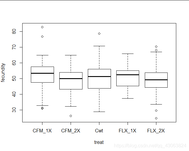
> ffa = read.csv("FFA.csv")
> str(ffa)
'data.frame':	252 obs. of  2 variables:
 $ treat    : Factor w/ 5 levels "CFM_1X","CFM_2X",..: 1 1 1 1 1 1 1 1 1 1 ...
 $ fecundity: num  47.6 41.2 52.8 58 56.8 55.6 52.4 47.4 44.6 32.8 ...
> boxplot(fecundity~treat, data=ffa)
2 Construct one-way anova model
Again, use lm() to construct your model. We need the basic model to test our assumptions and to be able to carry out the planned contrasts.
#Construct model
> fit.ffa = lm(fecundity~treat, data=ffa)
3 Assumptions of one-way anova
> par(mfrow=c(2,2))
> plot(fit.ffa)
> par(mfrow=c(1,1))
> shapiro.test(fit.ffa$residuals)

	Shapiro-Wilk normality test

data:  fit.ffa$residuals
W = 0.98871, p-value = 0.04608

> x <-fit.ffa$residuals
> y <-pnorm(summary(x), mean =mean(x, na.rm=TRUE), sd =sd(x, na.rm=TRUE))
> ks.test(x, y)

	Two-sample Kolmogorov-Smirnov test

data:  x and y
D = 0.5, p-value = 0.1068
alternative hypothesis: two-sided
> leveneTest(fit.ffa)
Levene's Test for Homogeneity of Variance (center = median)
       Df F value Pr(>F)
group   4  1.7948 0.1304
      247
 The QQ-plot looks fine and the Shapiro-Wilks test is only marginally non-significant. There is no evidence of differences in variance between groups. Assumptions are fulfilled.
4 Carry out planned contrast
The contrasts should sum to zero within a given comparison.
These values can be interpreted as part of an equation where we want to test if:
a)1CFM_1X -1CFM_2X + 0Cwt + 1FLX_1X –1FLX_2X = 0
b)1CFM_1X + 1CFM_2X + 0Cwt -1FLX_1X –1FLX_2X = 0
To construct this contrast matrix for use with glht(), use the following:
> plc = matrix(c(1, -1, 0, 1, -1,1, 1, 0, -1, -1),2,5, byrow=TRUE)
> rownames(plc) = c("1X vs. 2X", "CFM vs. FLX")
Now we can use the matrix to get our significance tests:
> result.plc = glht(fit.ffa, linfct =mcp(treat=plc))
> summary(result.plc)

	 Simultaneous Tests for General Linear Hypotheses

Multiple Comparisons of Means: User-defined Contrasts


Fit: lm(formula = fecundity ~ treat, data = ffa)

Linear Hypotheses:
                 Estimate Std. Error t value
1X vs. 2X == 0     6.0788     2.6326   2.309
CFM vs. FLX == 0   0.4663     2.6326   0.177
                 Pr(>|t|)
1X vs. 2X == 0      0.043 *
CFM vs. FLX == 0    0.980
---
Signif. codes:
0 ‘***’ 0.001 ‘**’ 0.01 ‘*’ 0.05 ‘.’ 0.1 ‘ ’ 1
(Adjusted p values reported -- single-step method)
You should find that there is a marginally significant difference in the first comparison, but no evidence of a difference in the second comparison. So there may be some evidence of dominance or inbreeding effects on female fecundity, but female-limited selection on the X chromosome does not seems in itself to have much of an effect on fecundity.
You might be thinking “But why not just use a regular one-way anova with posthoc comparisonsto test these hypotheses?”. That would actually be fine, but it wouldn’t be as powerful. Carrying out a set of posthoc comparisons on this dataset would entail a lot of separate tests, all of which have to be corrected for. That means you would have reduced power to detect a true effect, because you’d need to correct for a lot of irrelevant tests. Carrying out two separate t-tests (one for each comparison) would also be an acceptable alternative –as long as we correct for multiple testing! –and provide a similar level of statistical power.
5 Illustrate results
> mean.1X = mean(subset(ffa$fecundity, ffa$treat=="CFM_1X"|ffa$treat=="FLX_1X"))
> mean.2X = mean(subset(ffa$fecundity, ffa$treat=="CFM_2X"|ffa$treat=="FLX_2X"))
> SE.1X = SE(subset(ffa$fecundity, ffa$treat=="CFM_1X"|ffa$treat=="FLX_1X"))
> SE.2X = SE(subset(ffa$fecundity, ffa$treat=="CFM_2X"|ffa$treat=="FLX_2X"))
> fec.dat = data.frame(group=c("1X","2X"), mean.fec=c(mean.1X, mean.2X), SE=c(SE.1X, SE.2X))
> bp = barplot(mean.fec~group, data=fec.dat, col="#CCCCFF", xlab="Evolved X copy number", ylab="Fecundity", ylim=c(0,60))
> arrows(bp, fec.dat$mean.fec-fec.dat$SE, bp, fec.dat$mean.fec+fec.dat$SE, code=3, angle=90)

Kruskal-Wallis test
In cases where the assumptions of a one-way anova are not fulfilled, the Kruskal-Wallis test is a non-parametric alternative. It is used when we want to test the effect of a categorical predictor variable on a continuous or ordinal dependent variable, but does not assume normality of the residuals or homogeneity of variances.
1 Dataimport and exploration
> peas =read.csv("peas.csv")
> boxplot(len~treat, data=peas)

2 Construct one-way anova model and check assumptions
Use lm() to construct your model object, and test the assumptions of a one-way anova as before.
#Construct model
> fit.peas = lm(len~treat, data=peas)
#Check assumptions
#Independent measurements
> dwtest(fit.peas)

	Durbin-Watson test

data:  fit.peas
DW = 2.5511, p-value = 0.9239
alternative hypothesis: true autocorrelation is greater than 0

#Homogeneity of variances and normality of residuals
> par(mfrow=c(2,2))
> plot(fit.peas)
> par(mfrow=c(1,1))
> shapiro.test(fit.peas$residuals)

	Shapiro-Wilk normality test

data:  fit.peas$residuals
W = 0.96928, p-value = 0.2164

> x <-fit.peas$residuals
> y <-pnorm(summary(x), mean =mean(x, na.rm=TRUE), sd =sd(x, na.rm=TRUE))
> ks.test(x, y)

	Two-sample Kolmogorov-Smirnov test

data:  x and y
D = 0.6, p-value = 0.04226
alternative hypothesis: two-sided
We only have integer values for len, which means that the QQ-plot isn’t looking great. More worryingly, the variances do not seem to be equal across the treatment groups. A one-way anova isprobably not the best choice in this case.
3 Assumptions of Kruskal-Wallis test
The only assumption that needs to be fulfilled is that of independence of the observations. If you like, you can carry out a Durbin-Watson test, under the assumption that the data was collected in the order it is listed in the file. You should find no reason for concern
4 Get results of Kruskal-Wallis test
> kruskal.test(len~treat, data=peas)

	Kruskal-Wallis rank sum test

data:  len by treat
Kruskal-Wallis chi-squared = 38.437, df = 4,
p-value = 9.105e-08
It will confirm that there is a significant effect of the sugar treatments on pea section lengths.
5 Carry out non-parametric posthoc test
There are various options that could be used for carrying out a set of non-parametric posthoc tests on this dataset, such as the Dunn or Nemenyi tests for multiple comparisons. Since we’ve already talked about how to do a Wilcoxon signed ranks test, we’ll do pairwise Wilcoxon signed ranks tests with correction for multiple testing. There is a convenient function for this called pairwise.wilcox.test(), which even lets you specify the method of adjustment for multiple testing:
> pairwise.wilcox.test(peas$len, peas$treat, p.adjust.method="fdr")

	Pairwise comparisons using Wilcoxon rank sum test

data:  peas$len and peas$treat

   1g1f    2f      2g      2s
2f 1.00000 -       -       -
2g 0.10446 0.22894 -       -
2s 0.00034 0.00034 0.00043 -
c  0.00034 0.00034 0.00034 0.00098

P value adjustment method: fdr
6 Illustrate results
> peas$treat = factor(peas$treat,levels(peas$treat)[c(5,2:4,1)])
> hs = c("c","a","a","b","a")
> bx = boxplot(len~treat, data=peas, col="chartreuse", ylim=c(50,80), xlab="Sugar treatment", ylab="Pea section length")
> text(1:5, bx$stat[5,]+3, hs)
