pytorch神经网络
Imagine you are a radiologist working in this new high-tech hospital. Last week you got your first neural-network based model to assist you making diagnoses given your patients data and eventually improving your accuracy. But wait! Very much like us humans, synthetic models are never 100% accurate in their predictions. But how do we know if a model is absolutely certain or if it just barely surpasses the point of guessing? This knowledge is crucial for right interpretation and key for selecting appropriate treatment.
我想像一下您是在这家新高科技医院工作的放射科医生。 上周,您获得了第一个基于神经网络的模型,可帮助您根据患者数据进行诊断,并最终提高准确性。 可是等等! 就像我们人类一样,合成模型的预测永远不会100%准确。 但是,我们怎么知道一个模型是绝对确定的,还是仅仅超过了猜测点呢? 这些知识对于正确的解释至关重要,也是选择适当治疗方法的关键。
Assuming you’re more of an engineer: This scenario is also highly relevant for autonomous driving where a car constantly has to make decisions whether there is an obstacle in front of it or not. Ignoring uncertainties can get ugly real quick here.
假设您更多地是工程师:这种情况也与自动驾驶高度相关,在自动驾驶中,汽车必须不断做出决策,确定前方是否有障碍物。 在这里忽略不确定性会变得很丑陋。
If you are like 90% of the Deep Learning community (including past me) you just assumed that the predictions produced by the Softmax functionrepresent probabilities since they are neatly squashed into the domain [0,1]. This is a popular pitfall since these predictions generally tend to be overconfident. As we’ll see soon this behaviour is affected by a variety of architectural choices like the use of Batch Normalization or the number of layers.
如果您像90%的深度学习社区(包括我之前)一样,您只是假设Softmax函数产生的预测代表概率,因为它们被巧妙地压入了域[0,1]。 这是一个普遍的陷阱,因为这些预测通常倾向于过于自信。 我们很快就会看到,这种行为受到各种体系结构选择的影响,例如使用批处理规范化或层数。
You can find a interactive Google Colab notebook with all the code here.
您可以在此处找到带有所有代码的交互式Google Colab笔记本。
可靠性图 (Reliability Plots)
As we know now, it is desirable to output calibrated confidences instead of their raw counterparts. To get an intuitive understanding of how well a specific architecture performs in this regard, Realiability Diagramms are often used.
众所周知,希望输出经过校准的置信度而不是原始的置信度。 为了直观地了解特定体系结构在这方面的性能,经常使用Realiability Diagramms 。

Summarized in one sentence, Reliability Plots show how well the predicted confidence scores hold up against their actual accuracy. Hence, given 100 predictions each with confidence of 0.9, we expect 90% of them to be correct if the model is perfectly calibrated.
可靠性图表概括为一句话,显示了预测的置信度得分相对于其实际准确性的保持程度。 因此,给定100个预测,每个预测的置信度为0.9,如果模型经过完美校准,我们希望其中90%是正确的。
To fully understand what’s going on we need to dig a bit deeper. As we can see from the plot, all the confidence scores of the test set are binned into M=10 distinct bins [0, 0.1), [0.1, 0.2),…, [0.9, 1]. For each bin we can then calculate its accuracy
为了完全了解正在发生的事情,我们需要更深入地了解。 从图中可以看出,测试集的所有置信度得分都分为M = 10个不同的分箱[0,0.1),[0.1,0.2),…,[0.9,1]。 然后,对于每个垃圾箱,我们可以计算其准确性

and confidence
和信心

Both values are then visualized as a Bar plot with the identity line indicating perfect calibration.
然后将两个值显示为条形图,标识线表示完美校准。
指标 (Metrics)
Diagrams and plots are just one side of the story. In order to score a model based on its Calibration Error we need to define metrics. Fortunately, both metrics most often used here are really intuitive.
图表只是故事的一方面。 为了基于模型的校准误差对模型评分,我们需要定义指标。 幸运的是,这里最常用的两个指标都非常直观。
The Expected Calibration Error (ECE) simply takes a weighted average over the absolute accuracy/confidence difference.
预期校准误差(ECE)只是对绝对准确度/置信度差进行加权平均。

For safety critical applications, like described above, it may be useful to measure the maximum discrepancy between accuracy and confidence. This can be accomplished by using the Maximum Calibration Error (MCE).
对于如上所述的安全关键型应用,测量准确性和置信度之间的最大差异可能很有用。 这可以通过使用最大校准误差(MCE)来实现。
温度缩放 (Temperature Scaling)
We now want to focus on how to tackle this issue. While many solutions like Histogram Binning, Isotonic Regression, Bayesian Binning into Quantiles (BBQ) and Platt Scaling exist (with their corresponding extensions for multiclass problems), we want to focus on Temperature Scaling. This is due to the fact that it is the easiest to implement while giving the best results out of the other algorithms named above.
我们现在要集中精力于如何解决此问题。 尽管存在许多解决方案,例如直方图合并,等渗回归,将贝叶斯合并为分位数(BBQ)和普拉特缩放比例(以及针对多类问题的相应扩展),但我们希望专注于温度缩放比例。 这是由于这样的事实,它是最容易实现的,同时可以提供上述其他算法中最好的结果。
To fully understand it we need to take a step back and look at the outputs of a neural network. Assuming a multi-class problem, the last layer of a network outputs the logits zᵢ ∈ ℝ. The predicted probability can then be obtained using the Softmax function σ.
为了完全理解它,我们需要退后一步,看看神经网络的输出。 假设多类问题,网络的最后一层输出logitsŽᵢ∈ℝ。 然后可以使用Softmax函数σ获得预测的概率。

Temperature scaling directly works on the logits zᵢ (Not the predicted probabilities!!) and scales them using a single parameter T>0 for all classes. The calibrated confidence can then be obtained by
温度缩放直接作用于logitsŽᵢ(不是预测概率!!)和鳞它们使用的所有类的单个参数T> 0。 然后可以通过以下方式获得校准的置信度:
It is important to note that the parameter T is optimized with repect to the Negative-Log-Likelihood (NLL) loss on the validation set and the network’s parameters are fixed during this stage.
重要的是要注意,针对验证集上的负对数似然(NLL)损失,对参数T进行了优化,并且网络参数在此阶段是固定的。
结果 (Results)
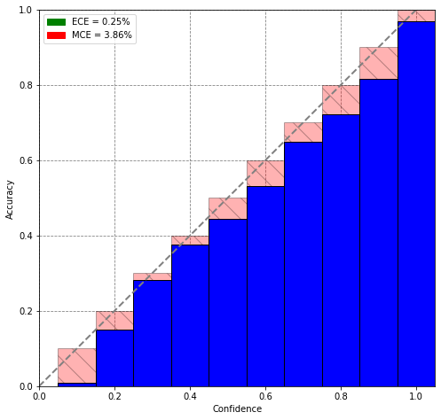
As we can see from the figure, the bars are now way closer to the identity line, indicating almost perfect calibration. We can also see this looking at the metrics. The ECE dropped from 2.10% to 0.25% and the MCE from 27.27% to 3.86%, which is a drastic improvement.
从图中可以看出,这些条现在更靠近标识线,表明校准几乎完美。 我们还可以查看指标。 ECE从2.10%下降到0.25%,MCE从27.27%下降到3.86%,这是一个巨大的进步。
在PyTorch中实施 (Implementation in PyTorch)
As promised, the implementation in PyTorch is rather straight forward.
如所承诺的,在PyTorch中的实现相当简单。
First we define the T_scaling method returning the calibrated confidences given a specific temperature T together with the logits.
首先,我们定义T_scaling方法,该方法返回给定特定温度T的校准置信度以及对数。
def T_scaling(logits, temperature):
  temperature = temperature.unsqueeze(1).expand(logits.size(0), logits.size(1))
  return logits / temperature
In the next step the parameter T has to be estimated using the LBGFS algorithm. This should only take a couple of seconds on a GPU.
在下一步中,必须使用LBGFS算法估算参数T。 在GPU上只需要几秒钟。
temperature = nn.Parameter(torch.ones(1).cuda())
criterion = nn.CrossEntropyLoss()
optimizer = optim.LBFGS([temperature], lr=0.001, max_iter=10000, line_search_fn='strong_wolfe')


logits_list = []
labels_list = []


for i, data in enumerate(tqdm(val_loader, 0)):
    images, labels = data[0].to(device), data[1].to(device)


    net.eval()
    with torch.no_grad():
      logits_list.append(net(images))
      labels_list.append(labels)


# Create tensors
logits_list = torch.cat(logits_list).to(device)
labels_list = torch.cat(labels_list).to(device)


def _eval():
  loss = criterion(T_scaling(logits_list, temperature), labels_list)
  loss.backward()
  return loss


optimizer.step(_eval)
You are welcome to play around in the Google Colab Notebook I created here.
欢迎您在我在此处创建的Google Colab笔记本中玩耍。
结论 (Conclusion)
As shown in this article, network calibration can be accomplished in just a few lines of code with drastic improvements. If there is enough interest I’m happy to discuss other approaches for model calibration in another Medium article. If you are interested in a deeper dive into this topic I highly recommend the Paper “On calibration of Neural Networks” by Guo et al..
如本文所示,网络校准只需几行代码即可完成,并进行了重大改进。 如果有足够的兴趣,我很乐意在另一篇Medium文章中讨论模型校准的其他方法。 如果您有兴趣深入研究该主题,我强烈推荐Guo等人的论文“关于神经网络的校准”。
Cheers!
干杯!
翻译自: https://medium.com/@lukas.huber1/neural-network-calibration-using-pytorch-c44b7221a61
pytorch神经网络