PyTorch 框架学习 更新中...

基础知识

Tensor 形式

import torch
from torch import tensor

Scalar:
通常就是一个数值

x = tensor(42.)
x # tensor(42.)

x.dim() # 0

2 * x # tensor(84.)

x.item() # 42.0

Vector
例如： [-5., 2., 0.]，在深度学习中通常指特征，例如词向量特征，某一维度特征等

v = tensor([1.5, -0.5, 3.0])
v # tensor([ 1.5000, -0.5000,  3.0000])

v.dim() # 1

v.size() # torch.Size([3])

Matrix
一般计算的都是矩阵，通常都是多维的

M = tensor([[1., 2.], [3., 4.]])
M
'''
tensor([[1., 2.],
        [3., 4.]])
'''

M.matmul(M)
'''
tensor([[ 7., 10.],
        [15., 22.]])
'''

tensor([1., 0.]).matmul(M)
'''
tensor([1., 2.])
'''

M * M
'''
tensor([[ 1.,  4.],
        [ 9., 16.]])
'''

tensor([1., 2.]).matmul(M) # tensor([ 7., 10.])

矩阵构造

torch.empty : 创建一个空矩阵

x = torch.empty(5, 3)
x
'''
tensor([[1.0469e-38, 9.3674e-39, 9.9184e-39],
        [8.7245e-39, 9.2755e-39, 8.9082e-39],
        [9.9184e-39, 8.4490e-39, 9.6429e-39],
        [1.0653e-38, 1.0469e-38, 4.2246e-39],
        [1.0378e-38, 9.6429e-39, 9.2755e-39]])
'''

torch.rand: 创建一个随机数矩阵

x = torch.rand(5, 3)
x
'''
tensor([[0.1452, 0.4816, 0.4507],
        [0.1991, 0.1799, 0.5055],
        [0.6840, 0.6698, 0.3320],
        [0.5095, 0.7218, 0.6996],
        [0.2091, 0.1717, 0.0504]])
'''

torch.zeros :初始化一个全零的矩阵

x = torch.zeros(5, 3, dtype=torch.long)
x
'''
tensor([[0, 0, 0],
        [0, 0, 0],
        [0, 0, 0],
        [0, 0, 0],
        [0, 0, 0]])
'''

torch.tensor: 自定义一个矩阵

x = torch.tensor([5.5, 3])
x # tensor([5.5000, 3.0000])

torch.randn_like :构造一个形状相同的随机数矩阵

x = x.new_ones(5, 3, dtype=torch.double)      

x = torch.randn_like(x, dtype=torch.float)    
x

矩阵的大小

x.size()

计算

直接使用+

y = torch.rand(5, 3)
x + y
'''
tensor([[ 0.6497, -0.5561,  2.2990],
        [ 0.5333,  0.4522,  2.1114],
        [-2.4560,  0.1690,  1.2198],
        [ 2.0695, -0.5944, -0.3466],
        [-0.2388,  0.5630,  0.8880]])
'''

torch.add : 加法操作

torch.add(x, y)
'''
tensor([[ 0.6497, -0.5561,  2.2990],
        [ 0.5333,  0.4522,  2.1114],
        [-2.4560,  0.1690,  1.2198],
        [ 2.0695, -0.5944, -0.3466],
        [-0.2388,  0.5630,  0.8880]])
'''

索引

x[:, 1]
'''
tensor([-1.1208, -0.0828, -0.4144, -0.7263,  0.1368])
'''

改变维度

view: 改变矩阵的维度

x = torch.randn(4, 4)
y = x.view(16)
z = x.view(-1, 8) # -1表示根据后面的值自动计算
print(x.size(), y.size(), z.size()) # torch.Size([4, 4]) torch.Size([16]) torch.Size([2, 8])

与numpy协同操作

numpy()转换为ndarray

a = torch.ones(5)
b = a.numpy()
b # array([1., 1., 1., 1., 1.], dtype=float32)

torch.from_numpy : 转换为tensor

import numpy as np
a = np.ones(5)
b = torch.from_numpy(a)
b # tensor([1., 1., 1., 1., 1.], dtype=torch.float64)

自动求导机制

定义一个可导的矩阵

import torch

#方法1
x = torch.randn(3,4,requires_grad=True)
x
'''
tensor([[-0.6812,  0.1245,  0.4627, -0.5860],
        [ 1.2594, -0.4262,  0.9005, -0.4189],
        [ 0.6924, -1.0704,  0.3465, -0.8244]], requires_grad=True)
'''

#方法2
x = torch.randn(3,4)
x.requires_grad=True
x
'''
tensor([[-1.0556,  1.2333, -0.9068,  1.1550],
        [-0.3289, -1.9466,  0.1828, -1.7511],
        [-0.4664,  0.5741,  0.9633, -0.3505]], requires_grad=True)
'''

b = torch.randn(3,4,requires_grad=True)
t = x + b
y = t.sum()
y # tensor(-2.1930, grad_fn=)

y.backward()
b.grad
'''
tensor([[1., 1., 1., 1.],
        [1., 1., 1., 1.],
        [1., 1., 1., 1.]])
'''
 
x.requires_grad, b.requires_grad, t.requires_grad  # (True, True, True)

链式求导法则

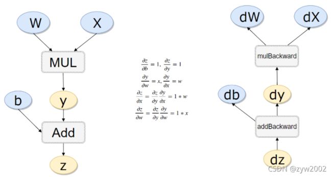
#计算流程
x = torch.rand(1)
b = torch.rand(1, requires_grad = True)
w = torch.rand(1, requires_grad = True)
y = w * x 
z = y + b 

x.requires_grad, b.requires_grad, w.requires_grad, y.requires_grad # (False, True, True, True)
x.is_leaf, w.is_leaf, b.is_leaf, y.is_leaf, z.is_leaf # (True, True, True, False, False)
# 计算反向传播
z.backward(retain_graph=True)#如果不清空会累加起来
w.grad # tensor([0.2456])
b.grad # tensor([8.])

线性回归模型

x_values = [i for i in range(11)]
x_train = np.array(x_values, dtype=np.float32)
x_train = x_train.reshape(-1, 1)
x_train.shape # (11, 1)

y_values = [2*i + 1 for i in x_values]
y_train = np.array(y_values, dtype=np.float32)
y_train = y_train.reshape(-1, 1)
y_train.shape # (11, 1)

# 线性回归其实就是一个不加激活函数的全连接层
import torch
import torch.nn as nn

class LinearRegressionModel(nn.Module):
    def __init__(self, input_dim, output_dim):
        super(LinearRegressionModel, self).__init__()
        self.linear = nn.Linear(input_dim, output_dim)  

    def forward(self, x):
        out = self.linear(x)
        return out

input_dim = 1
output_dim = 1

model = LinearRegressionModel(input_dim, output_dim)
model
'''
LinearRegressionModel(
  (linear): Linear(in_features=1, out_features=1, bias=True)
)
'''

# 指定好参数和损失函数
epochs = 1000
learning_rate = 0.01
optimizer = torch.optim.SGD(model.parameters(), lr=learning_rate)
criterion = nn.MSELoss()

# 训练模型
for epoch in range(epochs):
    epoch += 1
    # 注意转行成tensor
    inputs = torch.from_numpy(x_train)
    labels = torch.from_numpy(y_train)

    # 梯度要清零每一次迭代
    optimizer.zero_grad() 

    # 前向传播
    outputs = model(inputs)

    # 计算损失
    loss = criterion(outputs, labels)

    # 返向传播
    loss.backward()

    # 更新权重参数
    optimizer.step()
    if epoch % 50 == 0:
        print('epoch {}, loss {}'.format(epoch, loss.item()

# 测试模型预测结果
predicted = model(torch.from_numpy(x_train).requires_grad_()).data.numpy()
predicted

# 模型的保存与读取
torch.save(model.state_dict(), 'model.pkl')
model.load_state_dict(torch.load('model.pkl'))

使用GPU进行训练
只需要把数据和模型传入到cuda里面就可以了

import torch
import torch.nn as nn
import numpy as np


class LinearRegressionModel(nn.Module):
    def __init__(self, input_dim, output_dim):
        super(LinearRegressionModel, self).__init__()
        self.linear = nn.Linear(input_dim, output_dim)  

    def forward(self, x):
        out = self.linear(x)
        return out

input_dim = 1
output_dim = 1

model = LinearRegressionModel(input_dim, output_dim)


device = torch.device("cuda:0" if torch.cuda.is_available() else "cpu")
model.to(device)


criterion = nn.MSELoss()


learning_rate = 0.01

optimizer = torch.optim.SGD(model.parameters(), lr=learning_rate)

epochs = 1000
for epoch in range(epochs):
    epoch += 1
    inputs = torch.from_numpy(x_train).to(device)
    labels = torch.from_numpy(y_train).to(device)

    optimizer.zero_grad() 

    outputs = model(inputs)

    loss = criterion(outputs, labels)

    loss.backward()

    optimizer.step()

    if epoch % 50 == 0:
        print('epoch {}, loss {}'.format(epoch, loss.item()))

Hub模块

https://github.com/pytorch/hub
https://pytorch.org/hub/research-models

import torch
model = torch.hub.load('pytorch/vision:v0.4.2', 'deeplabv3_resnet101', pretrained=True)
model.eval()

torch.hub.list('pytorch/vision:v0.4.2')

# Download an example image from the pytorch website
import urllib
url, filename = ("https://github.com/pytorch/hub/raw/master/dog.jpg", "dog.jpg")
try: urllib.URLopener().retrieve(url, filename)
except: urllib.request.urlretrieve(url, filename)

# sample execution (requires torchvision)
from PIL import Image
from torchvision import transforms
input_image = Image.open(filename)
preprocess = transforms.Compose([
    transforms.ToTensor(),
    transforms.Normalize(mean=[0.485, 0.456, 0.406], std=[0.229, 0.224, 0.225]),
])

input_tensor = preprocess(input_image)
input_batch = input_tensor.unsqueeze(0) # create a mini-batch as expected by the model

# move the input and model to GPU for speed if available
if torch.cuda.is_available():
    input_batch = input_batch.to('cuda')
    model.to('cuda')

with torch.no_grad():
    output = model(input_batch)['out'][0]
output_predictions = output.argmax(0)

# create a color pallette, selecting a color for each class
palette = torch.tensor([2 ** 25 - 1, 2 ** 15 - 1, 2 ** 21 - 1])
colors = torch.as_tensor([i for i in range(21)])[:, None] * palette
colors = (colors % 255).numpy().astype("uint8")

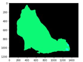
# plot the semantic segmentation predictions of 21 classes in each color
r = Image.fromarray(output_predictions.byte().cpu().numpy()).resize(input_image.size)
r.putpalette(colors)

import matplotlib.pyplot as plt
plt.imshow(r)
plt.show()

气温预测模型

import numpy as np
import pandas as pd 
import matplotlib.pyplot as plt
import torch
import torch.optim as optim
import warnings
warnings.filterwarnings("ignore")
%matplotlib inline

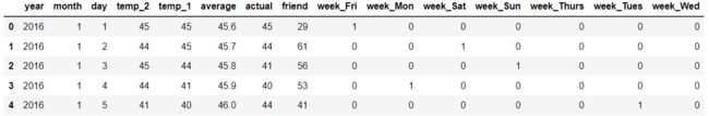
features = pd.read_csv('temps.csv')
features.head()

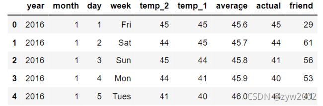
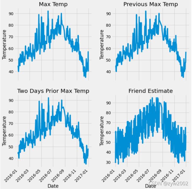
数据表中

year,moth,day,week分别表示的具体的时间
temp_2：前天的最高温度值
temp_1：昨天的最高温度值
average：在历史中，每年这一天的平均最高温度值
actual：这就是我们的标签值了，当天的真实最高温度
friend：这一列可能是凑热闹的，你的朋友猜测的可能值，咱们不管它就好了

print('数据维度:', features.shape) #  数据维度: (348, 9)

# 处理时间数据
import datetime

# 分别得到年，月，日
years = features['year']
months = features['month']
days = features['day']

# datetime格式
dates = [str(int(year)) + '-' + str(int(month)) + '-' + str(int(day)) for year, month, day in zip(years, months, days)]
dates = [datetime.datetime.strptime(date, '%Y-%m-%d') for date in dates]
dates[:5]
'''
[datetime.datetime(2016, 1, 1, 0, 0),
 datetime.datetime(2016, 1, 2, 0, 0),
 datetime.datetime(2016, 1, 3, 0, 0),
 datetime.datetime(2016, 1, 4, 0, 0),
 datetime.datetime(2016, 1, 5, 0, 0)]
'''

# 准备画图
# 指定默认风格
plt.style.use('fivethirtyeight')

# 设置布局
fig, ((ax1, ax2), (ax3, ax4)) = plt.subplots(nrows=2, ncols=2, figsize = (10,10))
fig.autofmt_xdate(rotation = 45)

# 标签值
ax1.plot(dates, features['actual'])
ax1.set_xlabel(''); ax1.set_ylabel('Temperature'); ax1.set_title('Max Temp')

# 昨天
ax2.plot(dates, features['temp_1'])
ax2.set_xlabel(''); ax2.set_ylabel('Temperature'); ax2.set_title('Previous Max Temp')

# 前天
ax3.plot(dates, features['temp_2'])
ax3.set_xlabel('Date'); ax3.set_ylabel('Temperature'); ax3.set_title('Two Days Prior Max Temp')

# 我的朋友
ax4.plot(dates, features['friend'])
ax4.set_xlabel('Date'); ax4.set_ylabel('Temperature'); ax4.set_title('Friend Estimate')

plt.tight_layout(pad=2)

# 独热编码
features = pd.get_dummies(features)
features.head(5)

# 标签
labels = np.array(features['actual'])

# 在特征中去掉标签
features= features.drop('actual', axis = 1)

# 名字单独保存一下，以备后患
feature_list = list(features.columns)

# 转换成合适的格式
features = np.array(features)

features.shape # (348, 14)

from sklearn import preprocessing
input_features = preprocessing.StandardScaler().fit_transform(features)
input_features[0]
'''
array([ 0.        , -1.5678393 , -1.65682171, -1.48452388, -1.49443549,
       -1.3470703 , -1.98891668,  2.44131112, -0.40482045, -0.40961596,
       -0.40482045, -0.40482045, -0.41913682, -0.40482045])
'''

构建网络模型

x = torch.tensor(input_features, dtype = float)

y = torch.tensor(labels, dtype = float)

# 权重参数初始化
weights = torch.randn((14, 128), dtype = float, requires_grad = True) 
biases = torch.randn(128, dtype = float, requires_grad = True) 
weights2 = torch.randn((128, 1), dtype = float, requires_grad = True) 
biases2 = torch.randn(1, dtype = float, requires_grad = True) 

learning_rate = 0.001 
losses = []

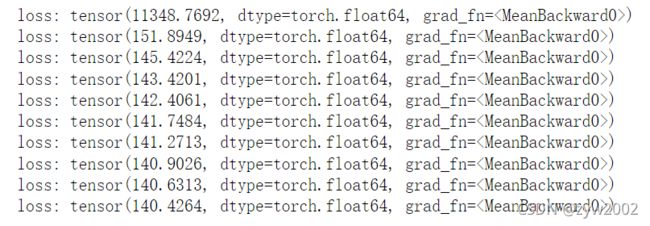
for i in range(1000):
    # 计算隐层
    hidden = x.mm(weights) + biases
    # 加入激活函数
    hidden = torch.relu(hidden)
    # 预测结果
    predictions = hidden.mm(weights2) + biases2
    # 通计算损失
    loss = torch.mean((predictions - y) ** 2) 
    losses.append(loss.data.numpy())
    
    # 打印损失值
    if i % 100 == 0:
        print('loss:', loss)
    #返向传播计算
    loss.backward()
    
    #更新参数
    weights.data.add_(- learning_rate * weights.grad.data)  
    biases.data.add_(- learning_rate * biases.grad.data)
    weights2.data.add_(- learning_rate * weights2.grad.data)
    biases2.data.add_(- learning_rate * biases2.grad.data)
    
    # 每次迭代都得记得清空
    weights.grad.data.zero_()
    biases.grad.data.zero_()
    weights2.grad.data.zero_()
    biases2.grad.data.zero_()

predictions.shape # torch.Size([348, 1])

构建更简单的网络模型

input_size = input_features.shape[1]
hidden_size = 128
output_size = 1
batch_size = 16
my_nn = torch.nn.Sequential(
    torch.nn.Linear(input_size, hidden_size),
    torch.nn.Sigmoid(),
    torch.nn.Linear(hidden_size, output_size),
)
cost = torch.nn.MSELoss(reduction='mean')
optimizer = torch.optim.Adam(my_nn.parameters(), lr = 0.001)

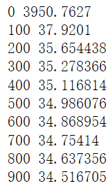
# 训练网络
losses = []
for i in range(1000):
    batch_loss = []
    # MINI-Batch方法来进行训练
    for start in range(0, len(input_features), batch_size):
        end = start + batch_size if start + batch_size < len(input_features) else len(input_features)
        xx = torch.tensor(input_features[start:end], dtype = torch.float, requires_grad = True)
        yy = torch.tensor(labels[start:end], dtype = torch.float, requires_grad = True)
        prediction = my_nn(xx)
        loss = cost(prediction, yy)
        optimizer.zero_grad()
        loss.backward(retain_graph=True)
        optimizer.step()
        batch_loss.append(loss.data.numpy())
    
    # 打印损失
    if i % 100==0:
        losses.append(np.mean(batch_loss))
        print(i, np.mean(batch_loss))

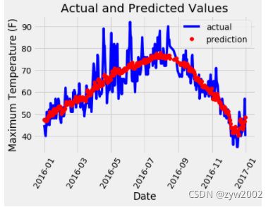
预测训练结果

x = torch.tensor(input_features, dtype = torch.float)
predict = my_nn(x).data.numpy()
# 转换日期格式
dates = [str(int(year)) + '-' + str(int(month)) + '-' + str(int(day)) for year, month, day in zip(years, months, days)]
dates = [datetime.datetime.strptime(date, '%Y-%m-%d') for date in dates]

# 创建一个表格来存日期和其对应的标签数值
true_data = pd.DataFrame(data = {'date': dates, 'actual': labels})

# 同理，再创建一个来存日期和其对应的模型预测值
months = features[:, feature_list.index('month')]
days = features[:, feature_list.index('day')]
years = features[:, feature_list.index('year')]

test_dates = [str(int(year)) + '-' + str(int(month)) + '-' + str(int(day)) for year, month, day in zip(years, months, days)]

test_dates = [datetime.datetime.strptime(date, '%Y-%m-%d') for date in test_dates]

predictions_data = pd.DataFrame(data = {'date': test_dates, 'prediction': predict.reshape(-1)}) 

# 真实值
plt.plot(true_data['date'], true_data['actual'], 'b-', label = 'actual')

# 预测值
plt.plot(predictions_data['date'], predictions_data['prediction'], 'ro', label = 'prediction')
plt.xticks(rotation = '60'); 
plt.legend()

# 图名
plt.xlabel('Date'); plt.ylabel('Maximum Temperature (F)'); plt.title('Actual and Predicted Values');

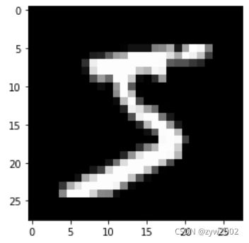
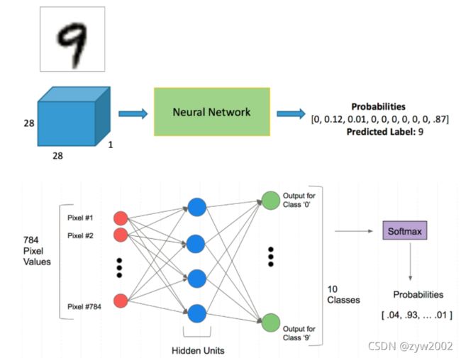
神经网络分类

%matplotlib inline
from pathlib import Path
import requests

DATA_PATH = Path("data")
PATH = DATA_PATH / "mnist"

PATH.mkdir(parents=True, exist_ok=True)

URL = "http://deeplearning.net/data/mnist/"
FILENAME = "mnist.pkl.gz"

if not (PATH / FILENAME).exists():
        content = requests.get(URL + FILENAME).content
        (PATH / FILENAME).open("wb").write(content)

import pickle
import gzip

with gzip.open((PATH / FILENAME).as_posix(), "rb") as f:
        ((x_train, y_train), (x_valid, y_valid), _) = pickle.load(f, encoding="latin-1")
from matplotlib import pyplot
import numpy as np

pyplot.imshow(x_train[0].reshape((28, 28)), cmap="gray")
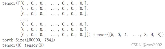
print(x_train.shape) # (50000, 784)

import torch

x_train, y_train, x_valid, y_valid = map(
    torch.tensor, (x_train, y_train, x_valid, y_valid)
)
n, c = x_train.shape
x_train, x_train.shape, y_train.min(), y_train.max()
print(x_train, y_train)
print(x_train.shape)
print(y_train.min(), y_train.max())

import torch.nn.functional as F

loss_func = F.cross_entropy

def model(xb):
    return xb.mm(weights) + bias
    
bs = 64
xb = x_train[0:bs]  # a mini-batch from x
yb = y_train[0:bs]
weights = torch.randn([784, 10], dtype = torch.float,  requires_grad = True) 
bs = 64
bias = torch.zeros(10, requires_grad=True)

print(loss_func(model(xb), yb))

创建一个model来更简化代码
必须继承nn.Module且在其构造函数中需调用nn.Module的构造函数
无需写反向传播函数，nn.Module能够利用autograd自动实现反向传播
Module中的可学习参数可以通过named_parameters()或者parameters()返回迭代器

from torch import nn

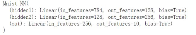
class Mnist_NN(nn.Module):
    def __init__(self):
        super().__init__()
        self.hidden1 = nn.Linear(784, 128)
        self.hidden2 = nn.Linear(128, 256)
        self.out  = nn.Linear(256, 10)

    def forward(self, x):
        x = F.relu(self.hidden1(x))
        x = F.relu(self.hidden2(x))
        x = self.out(x)
        return x
net = Mnist_NN()
print(net)

for name, parameter in net.named_parameters():
    print(name, parameter,parameter.size())

使用TensorDataset和DataLoader来简化

from torch.utils.data import TensorDataset
from torch.utils.data import DataLoader

train_ds = TensorDataset(x_train, y_train)
train_dl = DataLoader(train_ds, batch_size=bs, shuffle=True)

valid_ds = TensorDataset(x_valid, y_valid)
valid_dl = DataLoader(valid_ds, batch_size=bs * 2)

def get_data(train_ds, valid_ds, bs):
    return (
        DataLoader(train_ds, batch_size=bs, shuffle=True),
        DataLoader(valid_ds, batch_size=bs * 2),
    )

一般在训练模型时加上model.train()，这样会正常使用Batch Normalization和 Dropout
测试的时候一般选择model.eval()，这样就不会使用Batch Normalization和 Dropou

import numpy as np

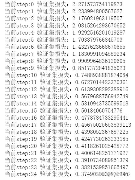
def fit(steps, model, loss_func, opt, train_dl, valid_dl):
    for step in range(steps):
        model.train()
        for xb, yb in train_dl:
            loss_batch(model, loss_func, xb, yb, opt)

        model.eval()
        with torch.no_grad():
            losses, nums = zip(
                *[loss_batch(model, loss_func, xb, yb) for xb, yb in valid_dl]
            )
        val_loss = np.sum(np.multiply(losses, nums)) / np.sum(nums)
        print('当前step:'+str(step), '验证集损失：'+str(val_loss))
        
from torch import optim
def get_model():
    model = Mnist_NN()
    return model, optim.SGD(model.parameters(), lr=0.001)
def loss_batch(model, loss_func, xb, yb, opt=None):
    loss = loss_func(model(xb), yb)

    if opt is not None:
        loss.backward()
        opt.step()
        opt.zero_grad()

    return loss.item(), len(xb)

train_dl, valid_dl = get_data(train_ds, valid_ds, bs)
model, opt = get_model()
fit(25, model, loss_func, opt, train_dl, valid_dl)