机器学习__03__机器学习之线性回归
文章目录
- 1.0 问题引入
-
- 1.1模型建立
- 1.2线性回归类型
- 2.0 线性回归描述
-
- 2.1普通线性回归
- 2.2Lasso回归
- 2.3岭回归
- 2.4ElasticNet回归
- 3.0线性回归案例之波士顿房价预测
- 4.0小结
在二十世纪二十年代以前,科学家基于传统牛顿力学、相对论等理论的成功,认为世界是由因果规律支配的,一切事物都严格遵守因果律和自然法则。也就是苹果会掉下来是因为有力在拉它,太阳在转也是因为有力在拉它。推导到最后就发现世界必须有一个源头提供原始的力,最终侧面证明了上帝的存在。
二十世纪二十年代,开创量子力学的哥本哈根学派科学家波尔、海森伯认则为认为世界上一切事物的发生都是不确定的,只能用概率也就是发生的可能性来描述事物运动规律。也就是说世间一切的事儿都符合于某种概率分布而不是因果,可以用概率模型来表示一切规律。
机器学习就是希望通过历史数据来找到事物背后的模式(pattern),而线性模型就是描述事物背后规律的一种方法,同时大部分的问题也是可以用线性模型来表示的。
1.0 问题引入
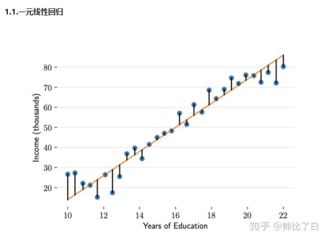
回归分析是一种预测性建模技术,主要用来研究因变量(yi)和自变量(xi)之间的关系,通常被用于预测分析、时间序列。
简单来说,回归分析就是使用曲线(直线是曲线的特例),或曲面来拟合某些已知的数据点,使数据点离曲线或曲面的距离差异达到最小。有了这样的回归曲线或者曲面后,我们就可以对新的自变量进行预测,即每一次输入一个自变量后,根据该回归曲线,或曲面,我们就可以得到一个对应的因变量,从而达到预测的目的。
1.1模型建立


1.2线性回归类型

2.0 线性回归描述
2.1普通线性回归
普通线性回归的原理如上面所述,在scikit-leam中通过linear model LinearRegression类进行了实现,下面介绍该类的主要参数和方法。
seikit-leam实现如下:
class sklearn.linear model.LinearRegression(fit_intercept=True,
normalize=False,n_jobs=1)
参数说明:
- fit_intercept:选择是否计算偏置常数b,默认是Tue,表示计算
- normalize:选择在拟合数据前是否对其进行归一化,默认为False,表示不进行归一化
- n_jobs:指定计算机并行工作时的CPU核数,默认是1。如果选择,表示使用所有可用的CU核。
属性说明:
- cof _:用于输出线性回归模型的权重向量w
- intercep_:列,用于输出线性国归模型的偏置常数b
方法:
- fit(X_train,y_train):在训练集(X train,.y train)上训练模型。
- score(X_test,y_test):返回模型在测试集(X_test,.y_test)上的预测准确率
2.2Lasso回归
Lesson回归就是在基本的线性回归基础上加上一个L1正则化项。前面讲过,L1正则化的主要作用是使各个特征的权重尽量接近于0,从而达到一种特征变量选择的效果。(正则化L1,可以将很多参数变为0,因此该方法可通过稀疏参数,降低负责度,从而弱化训练集噪声)。
Lasso回归在scikit--leam中是通过linear model..Lasso类实现的,下面介绍该类的

主要参数和方法:
scikit-learn实现如下:
class sklearn.linear model.Lasso (alpha=1.0,
								  fit intercept=True,
								  normalize=False,
								  precompute=False,
								  max iter=1000,
								  to1=0.0001,
								  warm start=False,
								  positive=False,
								  selection='cyclic')
参数:
- alpha:L1正则化项前面带的常数调节因子。
- fit intercept:选择是否计算偏置常数b,默认为True,表示计算。
- normalize:选择在拟合数据前是否对其进行归一化,默认为False,表示不进行归一化。
- precompute:选择是否使用预先计算的Gram矩阵来加快计算,默认为False。
- max_iter:设定最大迭代次数,默认为1000
- tol:设定判断迭代收敛的阈值,默认为0.0001
- wam_stat:设定是否使用前一次训练的结果继续训练,默认为False,表示每次从头开始训练。
- positive:默认为False;如果为True,则表示强制所有权重系数为正值。
- selection:每轮迭代时选择哪个权重系数进行更新,默认为cycle,表示从前往后依次选择;如果设定为random,则表示每次随机选择一个权重系数进行更新。
属性:
- coef_:用于输出线性回归模型的权重向量w
- intercept_:用于输出线性回归模型的偏置常数b
- n_iter_:用于输出实际迭代的次数
方法:
- fit(X_train,y_train:在训练集(X train,y_train)上训练模型
- score(X_test,y_test):返回模型在测试集(X_test,.y_test)上的预测准确率。
- predict(X):用训练好的模型来预测待预测数据集X,返回数据为预测集对应的预测结果
2.3岭回归
岭回归就是在基本的线性回归的基础上加上一个L2正则化项。前面讲过,L2正则化的主要作用是使各个特征的权重w尽衰减,从而在某种程度上达到一种特征变量选择的效果。
岭回归在scikit-leam中是通过linear_model.Ridge类实现的,下面介绍该类的主要参数和方法。
class sklearn.linear_model.Ridge (alpha=1.0,
							   	 fit_intercept=True,
								 normalize=False,
								 max_iter=None,
								 to1=0.001,
								 solver='auto')
参数:
-
alpha:L2正则化项前面带的常数调节因子
-
fit intercept:选择是否计算偏置常数b,默认为True,表示计算
-
normalize:选择在拟合数据前是否对其进行归一化,默认为False,表示不进行归一化
-
max iter:设定最大迭代次数,默认为1000
-
tol:设定判断迭代收敛的阈值,默认为0.0001
-
solver::指定求解最优化问题的算法,默认为auto,表示自动选择,其他可选项如下
选项如下。
- svd:使用奇异值分解来计算回归系数。
- cholesky:使用标准的scipy…linalg.solve函数来求解。
- sparse_cg:使用scipy…sparse…linalg…cg中的共轭梯度求解器求解。
- lsqr:使用专门的正则化最小二乘法scipy…sparse…linalg.lsq,速度是最快的。
- sg:使用随机平均梯度下降法求解。
属性:
-
coef_:用于输出线性回归模型的权重向量w
-
intercept_:用于输出线性回归模型的偏置常数b。
-
n_iter_:用于输出实际迭代的次数。
方法:
-
fit(X_train,y_train):在训练集(X_train,y_train)上训练模型
-
score(X_test,y_test):返回模型在测试集(X_test,y_test)上的预测准确率。
-
predict(X):用训练好的模型来预测待预测数据集X,返回数据为预测集对应的预测结果y。
2.4ElasticNet回归
ElasticNet回归(弹性网络回归)是将L1和L2正则化进行融合,即在基本的线性回归中加入下面的混合正则化项:
scikit-leam实现如下:
class sklearn.linear model.ElasticNet (alpha=1.0,
									  11_ratio=0.5,
									  fit_intercept=True,
                                      normalize=False,
                                      precompute=False,
                                      max_iter=1000,
                                      to1=0.0001,
                                      warm_start=False,
                                      positive=False,
                                      selection='cyclic')
参数:
- alpha:L1正则化项前面带的常数调节因子
- ll_ratio:ll_ratio参数就是上式中的p值,默认为0.5
- fit_intercept:选择是否计算偏置常数b,默认为True,表示计算
- normalize:选择在拟合数据前是否对其进行归一化,默认为False,表示不进行归一化
- precompute:选择是否使用预先计算的Gram矩阵来加快计算,默认为False
- max_iter:设定最大迭代次数,默认为l000
- tol:设定判断迭代收敛的阈值,默认为0.0001
- warm_start:设定是否使用前一次训练的结果继续训练,默认为False,表示每次从头开始训练
- positive:默认为False;如果为True,则表示强制所有权重系数为正值
- selection:每轮迭代时选择哪个权重系数进行更新,默认为cycle,表示从前往后依次选择;如果设定为random,则表示每次随机选择一个权重系数进行更新
属性
- coef:用于输出线性回归模型的权重向量w。
- intercept:用于输出线性回归模型的偏置常数b。
- n iter:用于输出实际迭代的次数。
方法
- fit(X_train,y_train):在训练集(X_train,y_train)上训练模型
- score(X_test,y_test):返回模型在测试集(X test,y test)上的预测准确率。
- predict(X):用训练好的模型来预测待预测数据集X,返回数据为预测集对应的预测结果y
3.0线性回归案例之波士顿房价预测
该数据集包含美国人口普查局收集的美国马萨诸塞州波士顿住房价格的有关信息, 数据集很小,只有506个案例。
数据集都有以下14个属性:
- CRIM–城镇人均犯罪率 ------【城镇人均犯罪率】
- ZN - 占地面积超过25,000平方英尺的住宅用地比例。 ------【住宅用地所占比例】
- INDUS - 每个城镇非零售业务的比例。 ------【城镇中非商业用地占比例】
- CHAS - Charles River虚拟变量(如果是河道,则为1;否则为0 ------【查尔斯河虚拟变量,用于回归分析】
- NOX - 一氧化氮浓度(每千万份) ------【环保指标】
- RM - 每间住宅的平均房间数------【每栋住宅房间数】
- AGE - 1940年以前建造的自住单位比例 ------【1940年以前建造的自住单位比例 】
- DIS -波士顿的五个就业中心加权距离 ------【与波士顿的五个就业中心加权距离】
- RAD - 径向高速公路的可达性指数 ------【距离高速公路的便利指数】
- TAX - 每10,000美元的全额物业税率 ------【每一万美元的不动产税率】
- PTRATIO - 城镇的学生与教师比例 ------【城镇中教师学生比例】
- B - 1000(Bk - 0.63)^ 2其中Bk是城镇黑人的比例 ------【城镇中黑人比例】
- LSTAT - 人口状况下降% ------【房东属于低等收入阶层比例】
- MEDV - 自有住房的中位数报价, 单位1000美元 ------【自住房屋房价中位数】

#波士顿房价预测
#波士顿房价数据于1978年开始统计,共包含506个样本点,每个样本都涵盖房屋的13种特征信息和对应的房屋价格


#(1)引入波士顿房价数据
from sklearn.datasets import load_boston                   #导入数据集
from sklearn.model_selection import train_test_split       #切分数据集
from sklearn.linear_model import ElasticNet                #运用ElasticNet回归模型训练和预测
import matplotlib.pyplot as plt                            #画图

boston=load_boston()
x=boston.data
y=boston.target

# (2)数据处理
unsF = []  # 次要特征下标
for i in range(len(name)):
    if name[i] == 'RM' or name[i] == 'PTRATIO' or name[i] == 'LSTAT' or name[i] == 'AGE' or name[i] == 'NOX' or name[i] == 'DIS' or name[i] == 'INDUS':
        continue
    unsF.append(i)
x = np.delete(x, unsF, axis=1)  # 删除次要特征

unsT = []  # 房价异常值下标
for i in range(len(y)):
    if y[i] > 46:
        unsT.append(i)
x = np.delete(x, unsT, axis=0)  # 删除样本异常值数据
y = np.delete(y, unsT, axis=0)  # 删除异常房价


print (x.shape)
print (y.shape)

#(3)数据集划分
x_train,x_test,y_train,y_test=train_test_split(x,y,train_size=0.7)

# (4)运用ElasticNet回归模型训练和预测
ElasticNet_clf=ElasticNet(alpha=0.1,l1_ratio=0.71)                #设置正则化调节因子 以及相关参数
ElasticNet_clf.fit(x_train,y_train.ravel())                       #在训练集中训练模型
ElasticNet_clf_score=ElasticNet_clf.score(x_test,y_test.ravel())  #返回模型在测试集上的准确率

print("模型得分:",ElasticNet_clf_score)
print("特征权重:",ElasticNet_clf.coef_)
print("偏置值:",ElasticNet_clf.intercept_)
print("迭代次数:",ElasticNet_clf.n_iter_)

#(5)画图
fig=plt.figure(figsize=(20,3)) #设置画布大小以及比例
axes=fig.add_subplot(1,1,1)    #画布为1X1即为一个模块
line1,=axes.plot(range(len(y_test)),y_test,'b',label='Actual_Value')  #实际值线条及图例

#用训练好的模型来预测待遇测数据集X,返回数据为预测集对应的结果
ElasticNet_clf_result=ElasticNet_clf.predict(x_test)

line2,=axes.plot(range(len(ElasticNet_clf_result)),ElasticNet_clf_result,'r--',label='ElasticNet_Predicted',linewidth=2) #预测值线条及图例

axes.grid()#包含表格
fig.tight_layout() #图例位置靠右
plt.legend(handles=[line1,line2]) #显示图例
plt.title('ElasticNet')           #设置标题
plt.show()

补充内容:其他线性回归的方式
import numpy as np
import numpy as np
from skimage.metrics import mean_squared_error
from sklearn import linear_model
from sklearn.linear_model import LinearRegression  # 导入线性模型
from sklearn.datasets import load_boston  # 导入数据集
from sklearn.metrics import r2_score
from sklearn.model_selection import train_test_split  # 导入数据集划分模块
from sklearn.linear_model import ElasticNet
from sklearn import preprocessing
import matplotlib.pyplot as plt
import matplotlib.pyplot as plt2

boston = load_boston()
x = boston['data']  # 影响房价的特征信息数据
y = boston['target']  # 房价
name = boston['feature_names']

# 数据处理
unsF = []  # 次要特征下标
for i in range(len(name)):
    if name[i] == 'RM' or name[i] == 'PTRATIO' or name[i] == 'LSTAT' or name[i] == 'AGE' or name[i] == 'NOX' or name[i] == 'DIS' or name[i] == 'INDUS':
        continue
    unsF.append(i)
x = np.delete(x, unsF, axis=1)  # 删除次要特征


unsT = []  # 房价异常值下标
for i in range(len(y)):
    if y[i] > 46:
        unsT.append(i)
x = np.delete(x, unsT, axis=0)  # 删除样本异常值数据
y = np.delete(y, unsT, axis=0)  # 删除异常房价

# 将数据进行拆分,一份用于训练,一份用于测试和验证
# 测试集大小为30%,防止过拟合
# 这里的random_state就是为了保证程序每次运行都分割一样的训练集和测试集。
# 否则,同样的算法模型在不同的训练集和测试集上的效果不一样。
x_train, x_test, y_train, y_test = train_test_split(x, y, test_size=0.3, random_state=0)


#线性回归模型
lf = LinearRegression()
lf.fit(x_train, y_train)  # 训练数据,学习模型参数
y_predict = lf.predict(x_test)  # 预测

# 岭回归模型
# rr = linear_model.Ridge()  # 模型岭回归
# rr.fit(x_train, y_train)  # 训练模型
# y_predict = rr.predict(x_test)  # 预测


# lasso模型
# lassr = linear_model.Lasso(alpha=.0001)
# lassr.fit(x_train, y_train)
# y_predict = lassr.predict(x_test)

# 与验证值作比较
error = mean_squared_error(y_test, y_predict).round(5)  # 平方差
score = r2_score(y_test, y_predict).round(5)  # 相关系数

# 绘制真实值和预测值的对比图
fig = plt.figure(figsize=(13, 7))
plt.rcParams['font.family'] = "sans-serif"
plt.rcParams['font.sans-serif'] = "SimHei"
plt.rcParams['axes.unicode_minus'] = False  # 绘图
plt.plot(range(y_test.shape[0]), y_test, color='red', linewidth=1, linestyle='-')
plt.plot(range(y_test.shape[0]), y_predict, color='blue', linewidth=1, linestyle='dashdot')
plt.legend(['真实值', '预测值'])
plt.title("190512213", fontsize=20)
error = "标准差d=" + str(error)+"\n"+"相关指数R^2="+str(score)
plt.xlabel(error, size=18, color="green")
plt.grid()
plt.show()

plt2.rcParams['font.family'] = "sans-serif"
plt2.rcParams['font.sans-serif'] = "SimHei"
plt2.title('190512213', fontsize=24)
xx = np.arange(0, 40)
yy = xx
plt2.xlabel(' truth ', fontsize=14)
plt2.ylabel(' predict ', fontsize=14)
plt2.plot(xx, yy)
plt2.scatter(y_test, y_predict, color='red')
plt2.grid()
plt2.show()
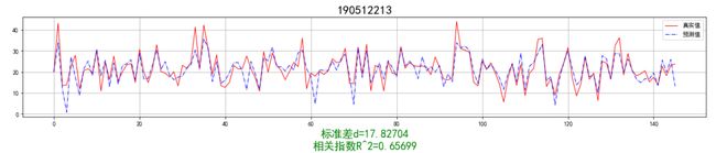

4.0小结
本章详细介绍了线性回归模型的基本原理和过程,展示了线性回归模型的scikit-leam实现,包括:普通线性回归、基于L1正则化的线性回归、基于L2正则化的岭回归、基于L1和L2正则化融合的ElasticNet回归四种,最后基于ElasticNetRegression在波士顿房价数据集上进行了实践展示,从结果来看,ElasticNet回归对房价的预测值和房价的真实值基本吻合。