Understanding Transductive Few-shot Learning

Image annotation can be a bottleneck for the applicability of machine learning when a costly expert annotation is needed. Some examples are medical imaging, astronomy, or botanics.

To alleviate this problem, few-shot classification aims to train classifiers from a small (few) number of samples (shot). A typical scenario is one-shot learning, with only one image per class. Another is zero-shot learning, where classes are given to the model in a different format. For instance, I could tell you “roses are red, the sky is blue” and you should be able to classify them without actually seeing any picture.

Recent works leverage unlabeled data to boost a few-shot performance. Some examples are label propagation and embedding propagation. These methods are in the “transductive” and “semi-supervised” learning (SSL) category. In this post, I will first overview the field of few-shot learning. Then I will explain transductive and SSL by using label propagation and embedding propagation as examples.
当需要昂贵的专家注释时，图像注释可能成为机器学习适用性的瓶颈。一些示例是医学成像，天文学或植物学。

为了缓解此问题，few-shot 分类旨在从少量（少量）样本（镜头）中训练分类器。一个典型的场景是一次性学习，每个班级只有一张图像。另一个是零镜头学习，其中以不同的格式为模型提供类。例如，我可以告诉您“玫瑰是红色，天空是蓝色”，您应该能够对其进行分类，而无需实际看到任何图片。

最近的工作利用未标记的数据来提高性能。一些示例是标签传播和嵌入传播。这些方法属于“转换式”和“半监督式”学习（SSL）类别。在这篇文章中，我将首先概述几次学习的领域。然后，我将以标签传播和嵌入传播为例，说明转导和SSL。

Few-shot Classification

In the typical few-shot scenario introduced by Vinyals et al., the model is presented with episodes composed of a support set and a query set. The support set contains information about the categories into which we want to classify the queries. For instance, the model could be given a picture of a computer and a tablet and from there it should be able to classify these two categories. In fact, models are usually given five categories (5-way), and one (one-shot) or five (five-shot) images per category. During training, the model is fed with these episodes and it has to learn to correctly guess the labels of the query set given the support set. The categories seen during training, validation, and testing, are all different. This way we know for sure that the model is learning to adapt to any data and not just memorizing information from the training set. Although most algorithms use episodes, different algorithm families differ in how to use these episodes to train the model. Next, I will introduce three families of algorithms: metric learning, gradient-based learning, and transfer learning.

在Vinyals等人介绍的典型的Few-shot学习场景中，该模型的情节由支持集和查询集组成。支持集包含有关我们要将查询分类到的类别的信息。例如，可以为模型提供一台计算机和一台平板电脑的图片，并从那里可以对这两个类别进行分类。实际上，模型通常被分为五个类别（5路），每个类别一个（一次拍摄）或五个（五个镜头）图像。在训练过程中，模型会饱受这些事件的困扰，并且必须学习在给定支持集的情况下正确猜测查询集的标签。在培训，验证和测试期间看到的类别都不同。这样，我们可以肯定地知道该模型正在学习适应任何数据，而不仅仅是记住训练集中的信息。尽管大多数算法使用情节，但不同的算法系列在如何使用这些情节训练模型方面有所不同。接下来，我将介绍三种算法：度量学习，基于梯度的学习和转移学习。

Metric learning approaches

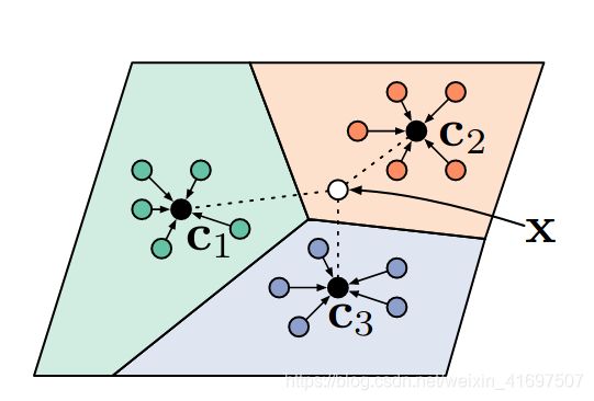
Currently, the simplest and most popular way of few-shot learning is metric learning. In this paradigm, the model learns to project images into a space where similar classes are close together given some distance metric, while different classes lay further apart. Perhaps the most well-known few-shot learning model is k-nearest neighbors, which would assign queries to the label of the closest supports. In fact, prototypical networks (Snell et al.), one of the most popular few-shot algorithms at this moment, is based on the same metric learning principle, see Figure 1.
当前，Few-shot Learning的最简单和最受欢迎的方式是度量学习。 在这种范例中，模型学习将图像投影到一个空间中，在给定距离度量的情况下，相似类彼此靠近，而不同类之间的距离则更远。 也许最著名的Few-shot Learning模型是k最近邻居，它将相邻查询的标签分配给查询。 实际上，原型网络（Snell等人）是目前最流行的Few-shot Learning算法之一，它基于相同的度量学习原理，请参见图1。

Figure 1. Prototypical networks. Images from the same category are averaged in the metric space in order to obtain a prototype that describes that category. Then a new image X is classified by choosing the label of the closest prototype. Credit. Snell et al.

图1.原型网络。 在度量空间中对来自同一类别的图像进行平均，以获得描述该类别的原型。 然后，通过选择最接近的原型的标签对新图像X进行分类。 信用。 Snell等。

Gradient-based approaches

Algorithms in this category, such as Model Agnostic Metalearning or MAML (Finn et al.), learn a good network initialization so that any problem can be solved by fine-tuning the model on a given support set. For each training iteration, MAML optimizes copies of the network parameters on multiple episodes at the same time and then updates the original weights by doing back-propagation through all these optimizations. MAML has inspired many posterior works such as Reptile, iMAML, or ANIL.
这一类的算法，例如不可知模型学习或MAML（Finn等人），学习了良好的网络初始化，因此可以通过在给定的支持集上微调模型来解决任何问题。 对于每次训练迭代，MAML都会同时优化多个情节上网络参数的副本，然后通过所有这些优化的反向传播来更新原始权重。 MAML启发了许多后继作品，例如Reptile，iMAML或ANIL。

Figure 2. Three versions of MAML.
θ is optimized to be close to the solutions of each individual episode. Credit (Rajeswaran et al.)

Transfer learning approaches

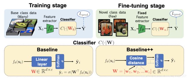
Recently, transfer learning approaches have become the new state-of-the-art for few-shot classification. Methods like Dynamic Few-Shot Visual Learning without Forgetting (Gidaris & Komodakis), pre-train a feature extractor in a first stage, and then, in a second stage, they learn to reuse this knowledge to obtain a classifier on new samples. Due to its success and simplicity, transfer learning approaches have been named “Baseline” on two recent papers (Chen et al., Dhillon et al.).
最近，转移学习方法已成为针对Few-shot 分类的最新技术。 无需忘记就可以进行动态少量快速视觉学习（Gidaris和Komodakis）之类的方法，在第一阶段对训练特征提取器进行了预训练，然后在第二阶段，他们学习了重用此知识以在新样本上获得分类器。 由于它的成功和简单性，最近两篇论文（Chen等人，Dhillon等人）将迁移学习方法称为“基线”。

Figure 3. A Closer Look At Few-shot Classification. The model follows the classic train and fine-tune pipeline of transfer learning. Credit Chen et al.
图3.细看Few-shot分类。 该模型遵循经典的培训和转移学习的精细调整流程。 陈等。

Needless to say, there are many works that are not cited here and deserve some time, as well as bayesian or generative methods. However, the purpose of this post is to introduce transductive few-shot learning, which comes next after this brief introduction to few-shot learning.
不用说，这里没有引用很多作品，还有一些时间，还有贝叶斯方法或生成方法。 但是，这篇文章的目的是介绍转瞬即逝的 few-shot学习，这是继对 few-shot learning的简短介绍之后。

Transductive Few-shot Learning

The most common classification scenario in machine learning is the inductive one (or not so, as you will see later…). In this scenario, we have to learn a function that produces a label for any given input. Differently, in the transductive scenario, the model has access to all the unlabeled data that we want to classify, and it only needs to produce labels for those samples (as opposed to every possible input sample). In practice, transduction is used as a form of semi-supervised learning, where we have some unlabeled samples from which the model can obtain extra information about the data distribution to make better predictions. In few-shot learning, transductive algorithms make use of all the queries in an episode instead of treating them individually. One possible criticism of this scenario is that there are usually 15 queries per class, and it is unrealistic that we get balanced unlabeled data in real life applications. As Nichol et al. point in their paper, note that many few-shot algorithms are already transductive thanks to batchnorm.

机器学习中最常见的分类方案是归纳法（或者不是，您将在后面看到……）。在这种情况下，我们必须学习一个为任何给定输入生成标签的函数。不同的是，在转导方案中，模型可以访问我们要分类的所有未标记数据，并且只需要为这些样本生成标签（而不是每个可能的输入样本）。在实践中，转导被用作半监督学习的一种形式，其中我们有一些未标记的样本，模型可以从中获取有关数据分布的额外信息，从而做出更好的预测。在few-shot learning中，转导算法会利用情节中的所有查询，而不是单独处理它们。对这种情况的一种可能的批评是，每个类通常有15个查询，并且在现实生活中的应用程序中获得平衡的未标记数据是不现实的。作为尼科尔等。在他们的论文中，请注意，由于batchnorm的缘故，许多很少使用的算法已经具有转导性。

Recently, transductive algorithms have increased in popularity in few-shot classification thanks to the work of Liu et al. who leverage a transductive algorithm called label propagation. So, what is label propagation?

最近，得益于Liu等人的工作，转导算法在 Few-shot分类中的流行度有所提高。 他们利用称为标签传播的转导算法。 那么，什么是标签传播？

Label Propagation

Label propagation (Zhu & Ghahramani) is an algorithm that consists in transmitting label information through the nodes of a graph, where nodes correspond to labeled and unlabeled samples. This graph is built based on some similarity metric between embeddings so nodes that are close in the graph are supposed to have similar labels. The main advantage with respect to other algorithms such as KNN is that label propagation respects the structure of the data. Here is an example I made:
标签传播（Zhu＆Ghahramani）是一种算法，该算法包括通过图的节点传输标签信息，其中节点对应于标记和未标记的样本。 此图是基于嵌入之间的某种相似性度量标准构建的，因此图中接近的节点应具有相似的标签。 相对于其他算法（例如KNN）的主要优点是标签传播尊重数据的结构。 这是我做的一个例子：

Figure 4. Label propagation. Circles are unlabeled nodes while triangles are labeled. The label propagation algorithm propagates label information through the nodes.

图4.标签传播。 圆形是未标记的节点，而三角形则是标记的。 标签传播算法通过节点传播标签信息。

Although this propagation algorithm is iterative, (Zhou et al.) proposed a closed-form solution. The algorithm is as follows:
尽管此传播算法是迭代的，但（Zhou等人）提出了一种封闭形式的解决方案。 算法如下：

1. Compute the similarity matrix
   W of the nodes. In this matrix Wi,j
   the similarity between the node and the node . The diagonal is zeroed to avoid self-propagation.

2. Then compute
   

the Laplacian matrix, which can be seen as a matrix representation of the graph.

3. Get the propagator matrix
   . Basically, this matrix tells you how much label information you have to transmit from one node to another.

4. Finally, given a matrix Y where each row is the one-hot encoding of a node, and most rows are made of 0s (unlabeled samples) while some contain a 1 in the corresponding class, the final labels
   are PY.

The matrix inverse is an expensive operation and makes it difficult to apply for large datasets, but luckily few-shot episodes are small. Thus, Liu et al. proposed a Transductive Propagation Network (TPN) for Few-shot Learning, shown in the Figure below:

矩阵逆运算是一项昂贵的操作，很难应用于大型数据集，但幸运的是，很少有几集是很小的。 因此，刘等。 提出了一种用于少拍学习的传导传播网络（TPN），如下图所示：

Figure 5. Transductive propagation network. Image features are extracted with a CNN. Then these features are used to build a graph with similarity matrix W. In order to have 0s for non-adjacent nodes a Radial Basis Function is used. is predicted by another neural network (). Credit: Liu et al.

The idea is that the labels of the support set get transmitted to the query set through the graph. This architecture turned out to be very effective, obtaining state-of-the-art results and inspiring new state-of-the-art methods such as embedding propagation.

这个想法是支持集的标签通过图形被传输到查询集。 事实证明，这种体系结构非常有效，可以获得最新的结果，并激发了诸如嵌入传播之类的最新技术。

Embedding Propagation

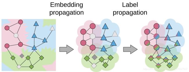
As explained by Chapelle et al., semi-supervised learning and transductive learning algorithms make three important assumptions on the data: smoothness, cluster, and manifold assumptions. In the recent embedding propagation paper published at ECCV2020, the authors build on the first assumption to improve transductive few-shot learning. Concretely, this assumption says that points that are close in embedding space must be close also in label space (similar points have similar labels). In order to achieve this smoothness, the authors applied the label propagation algorithm to propagate image feature information instead of label information as you can see in the next Figure:

Figure 6. Embedding Propagation is used to smooth the class representation manifold for label propagation.

This means nodes that are similar to each other become even closer to each other, increasing the density of the embedding space. As a result, label propagation applied on these new dense embeddings achieves higher performance:

图6.嵌入传播用于平滑用于标签传播的类表示流形。

这意味着彼此相似的节点变得更加接近，从而增加了嵌入空间的密度。 结果，应用于这些新的密集嵌入的标签传播实现了更高的性能：

Figure 7. Embedding Propagation performance on mini-Imagenet (a subset of ImageNet that is popular in few-shot classification). Both methods use the same neural architecture.

图7.在微型Imagenet（ImageNet的子集，在几次快照分类中很流行）上嵌入传播性能。 两种方法都使用相同的神经体系结构。

Moreover, the authors show that their method is also beneficial for semi-supervised learning and other transductive algorithms. For instance, they applied embedding propagation to the few-shot algorithm proposed by Gidaris et al. obtaining a 2% increase of performance in average. The authors provide PyTorch code in their github repository. You can use it in your model with only 3 extra lines of code:

import torch
from embedding_propagation import EmbeddingPropagation
ep = EmbeddingPropagation()
features = torch.randn(32, 32)
embeddings = ep(features)

Conclusions

Transductive learning has become a recurrent topic in few-shot classification. Here we have seen what is transductive learning and how it has improved the performance of few-shot algorithms. We have also seen some of its drawbacks, like the balance assumption of the unlabeled data. Finally, I have explained the recent embedding propagation algorithm to improve transductive few-shot classification and given some intuition on why it works.

跨性别学习已成为少拍分类中的经常性话题。 在这里，我们了解了什么是转导学习以及它如何提高一次性算法的性能。 我们还看到了它的一些缺点，例如未标记数据的余额假设。 最后，我解释了最近的嵌入传播算法，以改进转导性的few-shot分类，并给出了为何起作用的一些直觉。